DSpace at VNU: A phase decomposition approach and the Riemann problem for a model of two-phase flows

J. Math. Anal. Appl. 418 (2014) 569–594

Contents lists available at ScienceDirect

Journal of Mathematical Analysis and Applications
www.elsevier.com/locate/jmaa

A phase decomposition approach and the Riemann problem
for a model of two-phase flows
Mai Duc Thanh
Department of Mathematics, International University, Quarter 6, Linh Trung Ward, Thu Duc District,
Ho Chi Minh City, Viet Nam

a r t i c l e

i n f o

Article history:
Received 24 January 2013
Available online 13 April 2014
Submitted by H. Liu
Keywords:
Two-phase flow
Nonconservative
Phase decomposition
Generalized Rankine–Hugoniot
relations
Shock wave
Riemann problem

a b s t r a c t

We present a phase decomposition approach to deal with the generalized Rankine–
Hugoniot relations and then the Riemann problem for a model of two-phase flows.
By investigating separately the jump relations for equations in conservative form in
the solid phase, we show that the volume fractions can change only across contact
discontinuities. Then, we prove that the generalized Rankine–Hugoniot relations
are reduced to the usual form. It turns out that shock waves and rarefaction waves
remain on one phase only, and the contact waves serve as a bridge between the two
phases. By decomposing Riemann solutions into each phase, we show that Riemann
solutions can be constructed for large initial data. Furthermore, the Riemann
problem admits a unique solution for an appropriate choice of initial data.
© 2014 Elsevier Inc. All rights reserved.

1. Introduction
We consider in this paper the Riemann problem for the following model of two-phase flows, see [6],
∂t (αg ρg ) + ∂x (αg ρg ug ) = 0,
∂t (αg ρg ug ) + ∂x αg ρg u2g + pg

= pg ∂x αg ,

∂t (αs ρs ) + ∂x (αs ρs us ) = 0,
∂t (αs ρs us ) + ∂x αs ρs u2s + ps
∂t ρs + ∂x (ρs us ) = 0,

= −pg ∂x αg ,

x ∈ R, t > 0.

(1.1)

The system (1.1) is obtained from the full model of two-phase flows, see [4,6], namely the gas phase and

the solid phase, by assuming that the flow is isentropic in both phases. The first and the third equation of
(1.1) describe the conservation of mass in each phase; the second and the fourth equation of (1.1) describe
E-mail address:
/>0022-247X/© 2014 Elsevier Inc. All rights reserved.


570

M.D. Thanh / J. Math. Anal. Appl. 418 (2014) 569–594

the balance of momentum in each phase; the last equation of (1.1) is the so-called compaction dynamics
equation. Throughout, we use the subscripts g and s to indicate the quantities in the gas phase and in the
solid phase, respectively. The notations αk , ρk , uk , pk , k = g, s, respectively, stand for the volume fraction,
density, velocity, and pressure in the k-phase, k = g, s. The volume fractions satisfy
αs + αg = 1.

(1.2)

The system (1.1) has the form of nonconservative systems of balance laws
Ut + A(U )Ux = 0,

(1.3)

for U = (ρg , ug , ρs , us , αg ), and A(U ) is given at the beginning of Section 2. Weak solutions of such a
system can be understood in the sense of nonconservative products – a concept introduced by Dal Maso,
LeFloch and Murat [7]. In Section 2 we will brief this concept. Nonconservative systems can be used to
model multi-phase flows. Multi-phase flow models have attracted attention of many scientists not only for
the study theoretical problems such as existence, uniqueness, stability, and constructions of solutions, but
also numerical approximations of the solutions. In the case of two-phase flow models, there may be two
classes: the class of one-fluid models of two-phase flows and the class of two-fluid models of two-phase flows.

The situation is similar to multi-phase flow models. Both classes are of nonconservative form, but there
is a major difference between the two. That is, one-pressure models of two-phase flows are in general not
hyperbolic (see [12]), but two-pressure models of two-phase flows such as (1.1) are hyperbolic and strictly
hyperbolic except on a finite number of hyper-surfaces of the phase domain. Moreover, the characteristic
fields of two-phase flow models such as (1.1) have explicit forms. This raises the hope for the study of the
two-pressure models of two-phase flows: the theory of shock waves for hyperbolic systems of conservation
laws may be developed to study these hyperbolic models. In the numerical approximations, numerical
schemes employing an explicit form of characteristic fields, such as Roe-type schemes, can be implemented.
Therefore, the model (1.1), having applications in the modeling of the deflagration-to-detonation transition
(DDT) in granular explosives, is worth to study.
In this paper, we will present a method to construct solutions of the Riemann problem for the two-phase
flow model (1.1) using a phase decomposition approach. Observe that the construction of solutions of the
Riemann problem for hyperbolic systems when the solution vector has dimension larger than three is in
general very complicated. The solution vector of (1.1) has dimension five, so how to work through? It is very
interesting that in the system (1.1), four characteristic fields depend only on one phase, either gas or solid.
This allows the waves associated with these characteristic fields to change only in one phase and remain
constants in the other. This motivates us to propose a phase decomposition approach to build Riemann
solutions of (1.1), where waves associated with the 5th characteristic field will then be used as a “bridge”
to connect between the two phases. Precisely, we first investigate the impact of the jump conditions of the
conservation equations in the solid phase. This leads us to a crucial conclusion that across a discontinuity,
either the volume fractions remain constant, or the discontinuity is a contact wave. The first case yields
the usual form of the jump relations for shock waves. In the later case we can also point out that the jump
relations have the canonical form, by using a regularization method. Then, by a decomposition technique,
we can separate the Riemann solutions in each phase, where the two phases are now constraint to each other
via the solid contact. So, one can see that the solid contact in this method serves as a “bridge” to connect
between the group of solid components and the group of gas components of the Riemann solutions. As usual,
Riemann solutions are made from fundamental waves: shock waves, contact discontinuities, and rarefaction
waves. Shock waves and contact discontinuities are weak solutions in the sense of nonconservative products
and are of the usual form

M.D. Thanh / J. Math. Anal. Appl. 418 (2014) 569–594

U (x, t) =

U− ,
U+ ,

for x < σt,
for x > σt,

571

(1.4)

for some constant states U± and a constant shock speed σ. We will show that shock waves and contact waves
will be of path-independence. This allows us to determine uniquely these waves. The fact that the Riemann
solutions in this work can be understood in the sense of nonconservative product makes us believe that this
work will give a certain contribution to the theory of hyperbolic systems of balance laws in nonconservative
forms. Since these Riemann solutions are constructed in a deterministic way, they would be effectively used
in studying the front tracking method, the Glimm scheme, or Godunov-type schemes.
We observe that hyperbolic models in nonconservative forms have attracted many authors. The earlier
works concerning nonconservative systems were carried out in [13,14,18,10]. The Riemann problem for the
model of a fluid in a nozzle with discontinuous cross-section was solved in [15] for the isentropic case, and
in [21] for the non-isentropic case. The Riemann problem for shallow water equations with discontinuous
topography was solved in [16,17]. The Riemann problem for a general system in nonconservative form was
studied by [8]. In [3,19], some Riemann solutions of the Baer–Nunziato model of two-phase flows were
constructed. Two-fluid models of two-phase flows were studied in [12,20]. Numerical approximations for
two-phase flows were considered in [5,2,9,23,22,24]. See also the references therein.
The organization of this paper is as follows. Section 2 provides us with basic properties of the system

(1.1), and we recall the definition of weak solutions in the sense of nonconservative products. In Section 3 we
study the jump relations by using phase decomposition. We will show that the generalized Rankine–Hugoniot
relations can be reduced to the usual ones in the canonical form. Then, we define elementary waves that
make up Riemann solutions. In Section 4 we use phase decomposition to construct all possible Riemann
solutions, which can be done in each phase separately.
2. Preliminaries
2.1. Characteristic fields
When αs ≡ 0 or αg ≡ 0, the system (1.1) is reduced to the usual isentropic gas dynamics equations, and
the Riemann problem has been well-treated. For simplicity, we assume in the sequel that
αs > 0,

αg > 0.

(2.1)

This means that the flow always has exactly two phases. Furthermore, we will assume that the fluid in each
phase is isentropic and ideal, where the equation of state is given by
pk = κk ργkk ,

κk > 0, γk > 1, k = s, g.

(2.2)

For smooth solutions, under the assumptions (2.1), the system (1.1) is equivalent to the following system
∂t ρg + ug ∂x ρg + ρg ∂x ug +

ρg (ug − us )
∂x αg = 0,
αg

∂t ug + hg (ρg )∂x ρg + ug ∂x ug = 0,
∂t ρs + us ∂x ρs + ρs ∂x us = 0,
∂t us + hs (ρs )∂x ρs + us ∂x us +
∂t αg + us ∂x αg = 0,

pg − p s
∂x αg = 0,
αs ρs

x ∈ R, t > 0,

(2.3)


572

M.D. Thanh / J. Math. Anal. Appl. 418 (2014) 569–594

where hk is given by
hk (ρ) =

pk (ρ)
,
ρ

k = s, g.

From (2.3), choosing the dependent variable
U = (ρg , ug , ρs , us , αg ) ∈ R5 ,
we can re-write the system (1.1) as a system of balance laws in nonconservative form as

Ut + A(U )Ux = 0,

(2.4)

where
⎛

ug
⎜
⎜ hg (ρg )
⎜
A(U ) = ⎜ 0
⎜
⎝ 0
0

ρg
ug
0
0
0

0
0
0
0
us
ρs
hs (ρs ) us
0

0

ρg (ug −us )
αg

0
0

pg −ps
αs ρs

⎞
⎟
⎟
⎟
⎟.
⎟
⎠

us

Observe that if αs = 0, or αg = 0, then the matrix A(U ) is undefined.
Now, let us recall the concept of weak solutions of a nonconservative system of the form (2.4) for the
general case U ∈ RN in the sense of nonconservative products. Given a family of Lipschitz paths φ :
[0, 1] × RN × RN → RN satisfying
φ(0; U, V ) = U

φ(1; U, V ) = V,

∂s φ(s; U, V ) ≤ K|V − U |,

∂s φ(s; U1 , V1 ) − ∂s φ(s; U2 , V2 ) ≤ K |V1 − V2 | + |U1 − U2 | ,

(2.5)

for some constant K > 0, and for all s ∈ [0, 1], U, V, U1 , U2 , V1 , V2 ∈ RN . Let U be a function with bounded
variation in an interval [a, b] ⊂ R (in the following we will call it a BV-function for simplicity), then dU is
a Borel measure which coincides with the distributional derivative of U , i.e.,
b

b

U ϕ dx = −
a

ϕdU,

∀ϕ ∈ C0∞ [a, b]

a

(see [1]). The nonconservative product of a locally Borel bounded function and a Borel measure is given as
follows, see [7].
Definition 2.1. Let U = U (x), x ∈ [a, b], be a function with bounded variation. Then, the nonconservative
product μ := [g(U ) · dU ]φ of a locally Borel bounded function g : RN → RN by the vector-valued Borel
measure dU is a real-valued bounded Borel measure μ with the following properties:
(i) For any Borel set B, s.t. U is continuous on B:
μ(B) =

g(U )dU
B

(2.6)


M.D. Thanh / J. Math. Anal. Appl. 418 (2014) 569–594

573

(ii) For any x0 ∈ [a, b]:
1

g φ s; U (x0 −), U (x0 +) ∂s φ s; U (x0 −), U (x0 +) ds

μ(x0 ) =

(2.7)

0

Weak solutions can be understood in the sense of nonconservative products as follows, see [14].
Definition 2.2. A function U ∈ L∞ ∩ BVloc (R × R+ , RN ) is called a weak solution of the system in nonconservative form
Ut + A(U )Ux = 0,

U = U (x, t) ∈ RN

if the Borel measure
∂t U + A U (., t) ∂x U (., t)

(2.8)

φ

is equal to zero.
Let us consider now the hyperbolicity of the system (2.4). The characteristic equation of the matrix A(U )
in (2.4) is given by
(us − λ) (ug − λ)2 − pg (us − λ)2 − ps = 0,
which admits five roots as
λ1 (U ) = ug −

pg ,

λ2 (U ) = ug +

pg ,

λ3 (U ) = us −

ps ,

λ4 (U ) = us +

ps ,

λ5 (U ) = us .

(2.9)

The corresponding right eigenvectors can be chosen as
⎛
⎜

⎜
⎜
r1 (U ) = μ ⎜
⎜
⎝
⎛
⎜
⎜
r3 (U ) = ν ⎜
⎜
⎝
⎛

−ρg

⎞

⎟
pg (ρg ) ⎟
⎟
⎟,
0
⎟
⎠
0
0
⎞
0
⎟
0

⎟
−ρs ⎟
⎟,
ps (ρs ) ⎠
0

⎛
⎜
⎜
⎜
r2 (U ) = μ ⎜
⎜
⎝
⎛
⎜
⎜
r4 (U ) = ν ⎜
⎜
⎝

ρg

⎞

⎟
pg (ρg ) ⎟
⎟
⎟,
0
⎟

⎠
0
0
⎞
0
⎟
0
⎟
⎟,
ρs
⎟
ps (ρs ) ⎠
0
⎞

−(ug − us )2 ρg αs ps (ρs )
⎟
⎜
(ug − us )pg (ρg )ps (ρs )αs
⎟
⎜
2
⎟
r5 (U ) = ⎜
(p
(ρ
)
−
p
(ρ

))((u
−
u
)
−
p
(ρ
))α
g g
g
s
g ⎟,
g g
⎜ s s
⎠
⎝
0
2
((ug − us ) − pg (ρg ))αg αs ps (ρs )
where

(2.10)


574

M.D. Thanh / J. Math. Anal. Appl. 418 (2014) 569–594

Fig. 1. The projection of the phase domain in the (ρg , ug , us )-space and the projection of its intersection with the hyper-plane
us ≡ constant in the (ρg , ug )-plane.

2
μ=
ν=

pg (ρg )

pg (ρg )ρg + 2pg (ρg )

,

2 ps (ρs )
.
ps (ρs )ρs + 2ps (ρs )

It is not difficult to check that the eigenvectors ri , i = 1, 2, 3, 4, 5 are linearly independent. Thus, the system
is hyperbolic. Furthermore, it holds that
λ3 < λ5 < λ4 .
However, the eigenvalues λ5 may coincide with either λ1 or λ2 on a certain hyper-surface of the phase
domain, called the resonant surface. Due to the change of order of these eigenvalues, we set
Ω1 := U λ1 (U ) > λ5 (U ) ,
Ω2 := U λ1 (U ) < λ5 (U ) < λ2 (U ) ,
Ω3 := U λ2 (U ) < λ5 (U ) ,
Σ+ := U λ1 (U ) = λ5 (U ) ,
Σ− := U λ2 (U ) = λ5 (U ) .

(2.11)

The system is thus strictly hyperbolic in each domain Ωi , i = 1, 2, 3, but fails to be strictly hyperbolic on
the resonant surface

Σ := Σ+ ∪ Σ− .

(2.12)

Let us take an arbitrary and fixed value of the solid velocity us0 . It will be useful to consider the phase
domain in the hyper-plane us ≡ us0 . We denote by Gi , C± and C the projection in the (ρg , ug )-plane of the
intersection of the hyper-plane us ≡ us0 with the sets Ωi , Σ± and Σ, i = 1, 2, 3, respectively, see Fig. 1.
On the other hand, it is not difficult to verify that
Dλi (U ) · ri (U ) = 1,
Dλ5 (U ) · r5 (U ) = 0,

i = 1, 2, 3, 4,
(2.13)

so that the first, second, third, fourth characteristic fields (λi (U ), ri (U )), i = 1, 2, 3, 4, are genuinely nonlinear, while the fifth characteristic field (λ5 (U ), r5 (U )) is linearly degenerate.


M.D. Thanh / J. Math. Anal. Appl. 418 (2014) 569–594

575

2.2. Rarefaction waves
Next, let us look for rarefaction waves of the system (2.4). These waves are the continuous piecewisesmooth self-similar solutions of (1.1) associated with nonlinear characteristic fields, which have the form
U (x, t) = V (ξ),

ξ=

x
, t > 0, x ∈ R.
t

Substituting this into (2.4), we can see that rarefaction waves are solutions of the following initial-value
problem for ordinary differential equations
dV (ξ)
= ri V (ξ) ,
dξ

ξ ≥ λi (U0 ), i = 1, 2, 3, 4,

V λi (U0 ) = U0 .

(2.14)

Thus, the integral curve of the first characteristic field is given by
−2 pg (ρg )
dρg (ξ)
=
ρg (ξ) < 0,
dξ
pg (ρg )ρg + 2pg (ρg )
2 pg (ρg )
dug (ξ)
=
dξ
pg (ρg )ρg + 2pg (ρg )

pg (ξ) > 0,

dus (ξ)
dαg (ξ)

dρs (ξ)
=
=
= 0.
dξ
dξ
dξ

(2.15)

This implies that ρs , us , αg are constant through 1-rarefaction waves, ρg is strictly decreasing with respect to ξ, and ug is strictly increasing with respect to ξ. Moreover, since ρg is strictly monotone though
1-rarefaction waves, we can use ρg as a parameter of the integral curve
− pg (ρg )
dug
=
.
dρg
ρg

(2.16)

The integral curve (2.16) determines the forward curve of 1-rarefaction wave R1 (U0 ) consisting of all righthand states that can be connected to the left-hand state U0 using 1-rarefaction waves
ρg

R1 (U0 ):

ug = ω1 (ρg0 , ug0 ); ρg := ug0 −

pg (y)
y

dy,

ρg ≤ ρg0 ,

(2.17)

ρg0

where ρg ≤ ρg0 follows from the condition that the characteristic speed must be increasing through a
rarefaction fan.
Similarly, ρs , us , αg are constant through 2-rarefaction waves. The backward curve of 2-rarefaction wave
R2 (U0 ) consisting of all left-hand states that can be connected to the right-hand state U0 using 2-rarefaction
waves is given by
ρg

R2 (U0 ):

ug = ω2 (ρg0 , ug0 ); ρg := ug0 +
ρg0

pg (y)
y

dy,

ρg ≤ ρg0 .

(2.18)

M.D. Thanh / J. Math. Anal. Appl. 418 (2014) 569–594

576

In the same way, ρg , ug , αg are constant through 3- and 4-rarefaction waves. The forward curve of
3-rarefaction wave R3 (U0 ) consisting of all right-hand states that can be connected to the left-hand state
U0 using 3-rarefaction waves is given by
ρs

R3 (U0 ):

ps (y)
dy,
y

us = ω3 (ρs0 , us0 ); ρs := us0 −

ρs ≤ ρs0 .

(2.19)

ρs0

The backward curve of 4-rarefaction wave R4 (U0 ) consisting of all left-hand states that can be connected
to the right-hand state U0 using 4-rarefaction waves is given by
ρs

R4 (U0 ):

us = ω4 (ρs0 , us0 ); ρs := us0 +

ps (y)
dy,
y

ρs ≤ ρs0 .

(2.20)

ρs0

3. Phase decomposition for jump relations and elementary waves
Given a discontinuity of (1.1) of the form (1.4) in the sense of nonconservative product, this discontinuity
satisfies the generalized Rankine–Hugoniot relations for a given family of Lipschitz paths. We will show that
these generalized Rankine–Hugoniot relations will be reduced to the usual ones.
3.1. Phase decomposition for shock waves
Let us first consider the conservative equations in the solid phase of (1.1), which are the equation of
conservation of mass and the compaction dynamics equation. Since these equations are of conservative form,
the generalized Rankine–Hugoniot relations corresponding to any family of Lipschitz path must coincide
with the usual ones. This means that the following jump relations hold
−σ[αs ρs ] + [αs ρs us ] = 0,
−σ[ρs ] + [ρs us ] = 0,

(3.1)

where σ is the shock speed, [A] = A+ − A− , and A± denote the values on the right and left of the jump on
the quantity A. Eq. (3.1) can be rewritten as
αs ρs (us − σ) = 0,
ρs (us − σ) = 0,

or
ρs (us − σ) = M = constant,
M [αs ] = 0.

(3.2)

The second equation of (3.2) implies that either M = 0 or [αs ] = 0. Since ρs > 0, one obtains the following
conclusion: across any discontinuity (1.4) of (1.1)
– either [αs ] = 0,

or us = σ = constant.

(3.3)

It is derived from (3.3) that if [αs ] = 0, then the volume fractions remain constant across the discontinuity.
The system (1.1) is therefore reduced to the two independent sets of isentropic gas dynamics equations in
both phases


M.D. Thanh / J. Math. Anal. Appl. 418 (2014) 569–594

577

∂t ρg + ∂x (ρg ug ) = 0,
∂t (ρg ug ) + ∂x ρg u2g + pg = 0,
∂t ρs + ∂x (ρs us ) = 0,
∂t (ρs us ) + ∂x ρs u2s + ps = 0,

x ∈ R, t > 0.

(3.4)

This implies that ρs , us , αg are constant through 1- and 2-shock waves, while ρg , ug , αg are constant through
3- and 4-shock waves.
Given a left-hand state U0 , let us denote by Si (U0 ), i = 1, 3 the forward shock curves consisting of all
right-hand states U that can be connected to the left-hand state U0 by an i-Lax shock, i = 1, 3, and by
Sj (U0 ), j = 2, 4 the backward shock curves consisting of all left-hand states U that can be connected to the
right-hand state U0 by a j-Lax shock, j = 2, 4. These curves are given by:
ug = ω1 (ρg0 , ug0 ); ρg := ug0 −

(pg − pg0 )(ρg − ρg0 )
ρg0 ρg

1/2

S1 (U0 ):

ug = ω2 (ρg0 , ug0 ); ρg := ug0 +

(pg − pg0 )(ρg − ρg0 )
ρg0 ρg

1/2

S2 (U0 ):

us = ω3 (ρs0 , us0 ); ρs := us0 −

(ps − ps0 )(ρs − ρs0 )
ρs0 ρs

1/2

S3 (U0 ):

us = ω4 (ρs0 , us0 ); ρs := us0 +

(ps − ps0 )(ρs − ρs0 )
ρs0 ρs

1/2

S4 (U0 ):

,

ρg > ρg0 ,

,

ρg > ρg0 ,

,

ρs > ρs0 ,

,

ρs > ρs0 .

(3.5)

From (2.17)–(2.20) and (3.5), we can now define the forward wave curves issuing from U0 as
W1 (U0 ) = R1 (U0 ) ∪ S1 (U0 ),
W3 (U0 ) = R3 (U0 ) ∪ S3 (U0 ),

(3.6)

and the backward wave curves issuing from U0 by
W2 (U0 ) = R2 (U0 ) ∪ S2 (U0 ),
W4 (U0 ) = R4 (U0 ) ∪ S4 (U0 ).

(3.7)

These curves are parameterized in such a way that the velocity is given as a function of the density in each
phase, under the form u = ωi (U0 ; ρ), ρ > 0, i = 1, 2, 3, 4. It is not difficult to check that ω1 , ω3 are strictly
decreasing; and that ω2 , ω4 are strictly increasing.
Summarizing the above argument, we get the following result.
Lemma 3.1. Through an i-wave (shock or rarefaction), i = 1, 2, the quantities ρs , us , αg are constant.
Through a j-wave (shock or rarefaction), j = 3, 4, the quantities ρg , ug , αg are constant. The wave curves
Wi (U0 ), i = 1, 2, 3, 4, associated with the genuinely nonlinear characteristic fields issuing from a given state
U0 are given by (3.6) and (3.7).
The following result shows that the shock speeds of shock waves associated with nonlinear characteristic
fields may alter the order with the speed of contact waves.
Proposition 3.2. Consider the projection of the hyper-plane us ≡ us0 , for an arbitrarily fixed us0 , in the
(ρg , ug )-plane. The following conclusions hold.


578

M.D. Thanh / J. Math. Anal. Appl. 418 (2014) 569–594

#
(a) For any state U0 = (ρg0 , ug0 ) ∈ G1 , there exists a unique state denoted by U0# = (ρ#
g0 , ug0 ) ∈ S1 (U0 )∩G2 ,
#
#
u#
g0 > us0 such that the 1-shock speed σ1 (U0 , U0 ) coincides with the characteristic speed λ5 (U0 ). More
precisely,

σ1 U0 , U0# = λ5 U0# ,
σ1 (U0 , U ) > λ5 U0# ,

ρ ∈ ρ0 , ρ#
0 ,

σ1 (U0 , U ) < λ5 U0# ,

ρ ∈ ρ#
0 , +∞ .

(3.8)

(b) For any state U0 = (ρg0 , ug0 ) ∈ G3 , there exists a unique state denoted by U0 = (ρg0 , ug0 ) ∈ S2 (U0 )∩G2 ,
ug0 < us0 such that the 2-shock speed σ2 (U0 , U0 ) coincides with the characteristic speed λ5 (U0 ). More
precisely,
σ2 U0 , U0 = λ5 U0 ,
σ2 (U0 , U ) < λ5 U0 ,

ρ ∈ ρ0 , ρ0 ,

σ2 (U0 , U ) > λ5 U0 ,

ρ ∈ ρ0 , +∞ .

(3.9)

We omit the proof, since it is similar to the one of Proposition 2.4 [15].
3.2. Jump relations for contact waves
Let us now consider the second equation of (3.3) where [αs ] = 0. We will show that this is the case of a
contact discontinuity associated with the fifth characteristic field.
Theorem 3.3. Let U be a contact discontinuity of the form (1.4) associated with the linearly degenerate
characteristic field (λ5 , r5 ), that is, [αs ] = 0 and U± belongs to the same trajectory of the integral field of
the 5th characteristic field. Then, U is a weak solution of (1.1) in the sense of nonconservative products and
independent of paths. Moreover, this contact discontinuity U satisfies the jump relations in the usual form
us± = σ,
αg ρg (ug − us ) = 0,
(ug − us )2 + 2hg = 0,
[mug + αg pg + αs ps ] = 0,

(3.10)

where m is a constant given by
m = αg ρg (ug − us ).
Proof. Consider the integral curve corresponding to the 5th family passing through U−
dV (ξ)
= r5 V (ξ) ,
dξ

ξ ≥ ξ0 := λ5 (U− ),

V (ξ0 ) = U− .

(3.11)

A (unique) solution V = V (ξ) of (3.11) always exists on a certain interval [ξ0 , ξ1 ], where ξ1 > ξ0 . Let
U+ = V (ξ1 ).


M.D. Thanh / J. Math. Anal. Appl. 418 (2014) 569–594

579

Since [αs ] = 0, it follows from (3.2) that the first equation of (3.10) holds. Moreover, it is derived from
(2.13) that
dV (ξ)
dλ5 (V (ξ))
= Dλ5 V (ξ) ·
= Dλ5 V (ξ) · r5 V (ξ) ≡ 0.
dξ
dξ
This means that the 5th characteristic speed remains constant through trajectory of (3.11). Next, let
η : [ξ0 , ξ1 ] → R be any smooth function. We define a function
U (x, t) = V η(x − σt) = W (x − σt).

(3.12)

Then U is the classical solution of (2.4) with the smooth initial data
U (x, 0) = V ◦ η(x) = W (x),

x ∈ [ξ0 , ξ1 ].

Actually, it holds that, for ξ = x − σt
Ut + A(U )Ux = −Vξ (ξ)η σ + A V (ξ) Vξ (ξ)η (ξ)
= −Iσ + A V (ξ) Vξ (ξ)η (ξ)
= −Iλ5 V (ξ) + A V (ξ) r5 V (ξ) η (ξ) = 0,
where the last equation is deduced from the fact that λ5 remains constant across the trajectory (3.11). For
such a smooth solution U as in (3.12), the system (1.1) becomes
−σ(αg ρg ) + (αg ρg ug ) = 0,
−σ(αg ρg ug ) + αg ρg u2g + pg

= pg αg ,

−σ(αs ρs ) + (αs ρs us ) = 0,
−σ(αs ρs us ) + αs ρs u2s + ps

= −pg αg ,

−σρs + (ρs us ) = 0.

(3.13)

The first equation of (3.13) can be re-written in the divergence form as
αg ρg (ug − σ)

= 0,

(3.14)

which implies
αg ρg (ug − σ) ≡ m = constant.
The second equation of (3.13) is expressed as
αg ρg ug (ug − σ) + αg pg + pg αg = pg αg .
Using (3.14) and (3.15), and canceling the terms, we get from the last equation
(mug ) + αg pg = 0
or, since m is constant,

(3.15)


M.D. Thanh / J. Math. Anal. Appl. 418 (2014) 569–594

580

mug + αg pg = 0.
Using (3.15) in a reverse way, we obtain from the last equation
αg ρg (ug − σ) ug + αg pg = 0.
Canceling αg > 0 from the last equation to get
ρg (ug − σ)ug + pg = 0,
or
(ug − σ)ug + pg /ρg = 0.
The last equation yields the following equation in divergence form
(ug − σ)2 + 2hg

= 0,

hg = pg /ρg .

(3.16)

The third and the fifth equations of (3.13) are trivial, since σ = us ≡ constant, we discard them. Consider
the fourth equation of (3.13). Adding up the second equation to the fourth equation of (3.13) we obtain the
conservation of momentum of the mixture
−σ(αg ρg ug ) + αg ρg u2g + pg

− σ(αs ρs us ) + αs ρs u2s + ps

= 0.

The last equation can be simplified using (3.14) and that us = σ as follows
αg ρg ug (ug − σ) + (αg pg ) + αs ρs (us − σ) + (αs ps ) = 0,
or
(mug + αg pg + αs ps ) = 0.

(3.17)

We have established that the system (1.1) for the traveling wave solution is reduced to the system
(3.14)–(3.17):
αg ρg (ug − σ)

= 0,

(ug − σ)2 + 2hg

= 0,

(mug + αg pg + αs ps ) = 0,

(3.18)

where m is given by (3.15). Since (3.18) has a divergence form, it is independent of paths, if U is considered
as a weak solution in the sense of nonconservative products.
Now, let ηε be a sequence of smooth functions such that
ηε (x) →

ξ0 ,
ξ1 ,

for x < 0,
for x > 0,

as ε → 0.

(3.19)

Then, it holds that
Wε (x) = V ◦ ηε (x) → W0 (x) =

V (ξ0 ) = U− ,
V (ξ1 ) = U+ ,

for x < 0,
for x > 0.

(3.20)


M.D. Thanh / J. Math. Anal. Appl. 418 (2014) 569–594

581

As seen in the above argument, we obtain the sequence of corresponding smooth solutions Uε (x, t) =
Wε (x − σt) = V ◦ ηε (x − σt) of (1.1) that satisfy Eqs. (3.18). Let U still stand for Uε (x, t) in (3.18). Then,
passing to the limit of (3.18) for U = Uε (x, t) as ε → 0, we obtain the jump relations (3.10). Due to
the stability result of weak solutions in the sense of nonconservative products (see Theorem 2.2 [7]), the
function of the form (1.4), where the jump relations (3.10) hold, is a weak solution of the system (1.1) and
independent of paths. ✷
In the sequel, we fix one state U0 and look for any state U that can be connected with U0 by a contact
discontinuity. As seen above, the state U satisfies the equations
αg ρg (ug − us ) = αg0 ρg0 (ug0 − us ) := m,
(ug − us )2 + 2hg = (ug0 − us0 )2 + 2hg0 ,

(3.21)

and
ps =

αs0 ps0 − [mug + αg pg ]
.
αs

(3.22)

The quantities in the gas phase can be found using (3.21). Then, the solid pressure is given by (3.22), and
therefore the solid density can be calculated by using the equation of state (2.2).
3.3. Contact waves and admissibility criterion
Not all the jumps satisfying (3.10) are admissible. In the rest of this section we will investigate properties
of contact waves as well as the admissibility criterion for contact discontinuities.
For simplicity, in the rest of this section we will drop the subindex “g” for the quantities in the gas phase.

It follows from (3.21) that the gas density is a root of the nonlinear algebraic equation
F (U0 , ρ, α) := sgn(u0 − us ) (u0 − us )2 −

1/2

2κγ γ−1
ρ
− ργ−1
0
γ−1

ρ−

α0 (u0 − us )ρ0
= 0.
α

(3.23)

Let us investigate properties of the function F (U0 , ρ, α). First, the domain of this function is given by
(u0 − us )2 −

2κγ γ−1
ρ
− ργ−1
≥ 0.
0
γ−1

That is

ρ ≤ ρ¯(U0 ) :=

γ−1
(u0 − us )2 + ργ−1
0
2κγ

1
γ−1

.

A straightforward calculation shows that
2κγ
(ργ−1 − ργ−1
) − κγργ−1
(u0 − us )2 − γ−1
∂F (U0 , ρ; α)
0
=
.
2κγ
∂ρ
((u0 − us )2 − γ−1
(ργ−1 − ργ−1
))1/2
0

Consider first the case u0 − us > 0. Then, the last expression yields
∂F (U0 , ρ; α)

> 0,
∂ρ

ρ < ρmax (ρ0 , u0 ),

∂F (U0 , ρ; α)
< 0,
∂ρ

ρ > ρmax (ρ0 , u0 ),


582

M.D. Thanh / J. Math. Anal. Appl. 418 (2014) 569–594

where
ρmax (ρ0 , u0 ) :=

2
γ−1
(u0 − us )2 +
ργ−1
κγ(γ + 1)
γ+1 0

1
γ−1

.

(3.24)

The values of F at the limits are given by
F (U0 , ρ = 0, α) = F (U0 , ρ = ρ¯, α) = −

α0 (u0 − us )ρ0
< 0.
α

Thus, the function ρ → F (U0 , ρ; α) admits a root if and only if the maximum value is non-negative:
F (U0 , ρ = ρmax , α) ≥ 0.
In other words,
α0 ρ0 |u0 − us |
α ≥ αmin (U0 ) := √
.
γ+1
2
κγρmax
(ρ0 , u0 )

(3.25)

Similar argument can be made for u0 − us < 0.
The following lemma characterizes the properties of roots of Eq. (3.23).
Lemma 3.4. (i) The function F (U0 , ρ, α) in (3.23) admits a zero if and only if a ≥ αmin (U0 ). In this case,
F (U0 , ρ, α) admits two distinct zeros, denoted by ρ = ϕ1 (U0 , α), ρ = ϕ2 (U0 , α) such that
ϕ1 (U0 , α) ≤ ρmax (U0 ) ≤ ϕ2 (U0 , α)

(3.26)

the equality in (3.26) holds only if α = αmin (U0 ).
(ii) The state (ϕ1 (U0 , α), u = us + m/αϕ1 (U0 , α)) ∈ G1 if u0 > us , and the state (ϕ1 (U0 , α),
u = us + m/αϕ1 (U0 , α)) ∈ G3 if u0 < us ; the state (ϕ2 (U0 , α), u = us + m/αϕ2 (U0 , α)) ∈ G2 .
(iii)
– If α > α0 , then
ϕ1 (U0 , α) < ρ0 < ϕ2 (U0 , α).
– If α < α0 , then
ρ0 < ϕ1 (U0 , α)

for (ρ0 , u0 ) ∈ G1 ∪ G3 ,

ρ0 > ϕ2 (U0 , α)

for (ρ0 , u0 ) ∈ G2 .

(iv) Given us α, and let αmin (ρ, u) be defined as in (3.25). The following conclusions hold
αmin (ρ, u) < α,

(ρ, u) ∈ Gi , i = 1, 2, 3,

αmin (ρ, u) = α,

(ρ, u) ∈ C,

αmin (ρ, u) = 0,

u = 0.

The proof of Lemma 3.4 is omitted, since it is similar to the ones in [15].

Arguing similarly as in [15], one can construct a two-parameter family of solutions using shock waves,
rarefaction waves and contact discontinuities. This is because there are two possible choices of contact


M.D. Thanh / J. Math. Anal. Appl. 418 (2014) 569–594

583

discontinuities, as seen by Lemma 3.4. Therefore, to select a unique stationary wave, we need the following
admissibility criterion. Observe that the equations of (3.21) also define a curve
ρ → α = α(U− , ρ),

(3.27)

where U− = U0 and ρ varies between ρ± . We will postulate the following admissibility criterion for contact
waves.
(MC) Through any contact wave connecting U± , the volume fraction α given by (3.27) as a function of ρ
must vary monotonically in ρ between the two values ρ− and ρ+ . Furthermore, the total variation of
the volume fraction α of any Riemann solution must not exceed |αR − αL |.
A similar criterion was used in [15,21,10,11]. Given us , U0 = (ρ0 , u0 ), α0 , α, we denote by
Υ (U0 , α0 , α) = (ρ, u, α)
a state on the other side of the 5-contact wave from (ρ0 , u0 , α0 ) satisfying the (MC) criterion. In view of
Lemma 3.4, Υ (U0 , α0 , α) is a single point except on the resonant surface, where it consists of two points.
In discussing about the location of point sin the (ρ, u)-plane, we still refer to Υ (U0 , α0 , α) as its projection
onto this plane. The location of Υ (U0 , α0 , α) is given in the following lemma.
Lemma 3.5. Given us , U0 = (ρ0 , u0 ), α0 , α, let
Υ (U0 , α0 , α) = (ρ, u, α)
be a state on the other side of the 5-contact wave from (ρ0 , u0 , α0 ) satisfying the (MC) criterion. It holds
that
(i) If U0 ∈ G1 ∪ G3 , then the admissible 5-contact satisfying the (MC) criterion corresponds to the zero

ϕ(U0 , α) = ϕ1 (U0 , α) defined by Lemma 3.4. This means that Υ (U0 , α0 , α) ∈ G1 ∪ G3 .
(ii) If U0 ∈ G2 , then the admissible 5-contact satisfying the (MC) criterion corresponds to the zero
ϕ(U0 , α) = ϕ2 (U0 , α) defined by Lemma 3.4. This means that Υ (U0 , α0 , α) ∈ G2 .
(iii) It holds that
Υ U0 , α0 , αmin (U0 ) ∈ C+ ,

u0 > us ,

Υ U0 , α0 , αmin (U0 ) ∈ C− ,

u0 < us .

Proof. Since the proofs of (i) and (ii) are similar to the ones of Lemma 4.1 in [15], they are omitted.
For any given U0 = (ρ0 , u0 ) and α0 , according to the part (i) of Lemma 3.4, it holds that
ϕ1 (U0 , α) = ρmax (U0 ) = ϕ2 (U0 , α).
This means that the states on the other side of the 5-contacts from U0 with gas volume fraction α0 to
a state with gas volume fraction αmin (U0 ) coincide and so admissible. In our notations, it is denoted by
Υ (U0 , α0 , αmin (U0 )). According to the part (ii), the state Υ (U0 , α0 , αmin (U0 )) must be on the curve C.
Furthermore, since the state Υ (U0 , α0 , αmin (U0 )) and U0 must lie on the same side with respect to the line
u = us in the (ρ, u)-plane, the conclusion follows. ✷
The above argument leads to defining elementary waves of the system (1.1), which make up solutions of
the Riemann problem.


M.D. Thanh / J. Math. Anal. Appl. 418 (2014) 569–594

584

Definition 3.6. (a) (Elementary waves) The elementary waves of the system (1.1) are
• i-Lax shock waves, i = 1, 2, 3, 4;

• i-rarefaction waves, i = 1, 2, 3, 4;
• admissible 5-contact waves satisfying the criterion (MC).
(b) (Riemann solutions) Riemann solutions of (1.1) are made of elementary waves and are constraint
with the criterion (MC).
4. Solving the Riemann problem via phase decomposition
4.1. Notations
Throughout this section, we will use the following notations:
(i) Wk (Ui , Uj ) (Sk (Ui , Uj ), Rk (Ui , Uj )) denotes a k-wave (k-shock, or k-rarefaction wave, respectively) connecting the left-hand state Ui to the right-hand state Uj ;
(ii) Wm (Ui , Uj )⊕Wn (Uj , Uk ) indicates that there is an m-wave from the left-hand state Ui to the right-hand
state Uj , followed by an n-wave from the left-hand state Uj to the right-hand state Uk .
4.2. Phase decomposition
Recall from Lemma 3.1 that
– Through i-Lax shock waves and i-rarefaction waves, i = 1, 2, the quantities in the solid phase ρs , us and
αs remain constant;
– Through j-Lax shock waves and j-rarefaction waves, j = 3, 4, the quantities in the gas phase ρg , ug and
αg remain constant.
Clearly, the fact that the gas volume fraction remains constant is the same as that the solid volume
fraction remains constant. Only 5-contacts involve quantities in both phases, and so the 5-contacts conserve
as a “bridge” to provide a connection between the two phases. This suggests us that we can consider the
wave structure in each phase separately. In other words, we use a phase decomposition approach to treat
the Riemann problem. Without any confusion, when considering separately a phase, we still use the letter
U to denote a state in that phase.
Precisely, quantities in the solid phase involve only in the 3rd, 4th and 5th characteristic fields, where
λ3 (U ) < λ5 (U ) < λ4 (U ),
for all U in the phase domain. Thus, solid components in any Riemann solution involve only in these 3
families of waves which are separated by four constant states UL , V± = (ρs± , us± ), UR , as illustrated by
Fig. 2. One has in the solid phase
V− = (ρs− , us− ) ∈ W3 (UL ),

V+ = (ρs+ , us+ ) ∈ W4 (UR ).

(4.1)

Therefore, since us remains constant across the 5-contact, it holds that
us− = ω3 (ρsL , usL ); ρs− = us ,
us+ = ω4 (ρsR , usR ); ρs+ = us ,
where ω3 , ω4 are given by (2.19)–(2.20) and (3.5).

(4.2)


M.D. Thanh / J. Math. Anal. Appl. 418 (2014) 569–594

585

Fig. 2. Solid components of a Riemann solution in the (x, t)-plane.

Fig. 3. Case 1: gas components of a Riemann solution in the (x, t)-plane.

Quantities in the gas phase also involve only in the 3 families of waves from the 1st, 2nd, and 5th
characteristic fields. However, although
λ1 (U ) < λ2 (U ),
for all U in the phase domain, the values λ5 (U ) can be in any order with λ1 (U ) and λ2 (U ). This requires
us to consider several cases as in the following.
Case 1: the contact wave lies between the two nonlinear waves This case represents a situation where a
5-contact wave lies in the middle region between a 1-wave and a 2-wave, see Fig. 3. Since
U− = (ρg− , ug− ) ∈ W1 (UL ),

U+ = (ρg+ , ug+ ) ∈ W2 (UR ),

(4.3)

it holds that
ug− = ω1 (ρgL , ugL ); ρg− ,
ug+ = ω2 (ρgR , ugR ); ρg+ ,

(4.4)

where ω1 , ω2 are given by (2.17)–(2.18) and (3.5). From two equations in (4.2), two equations in (4.4), and
two equations in (3.21) determine the 5 quantities
ρg± ,

ug± ,

us .

Observe that this is an over-determined system, since us± = us .


586

M.D. Thanh / J. Math. Anal. Appl. 418 (2014) 569–594

Fig. 4. Case 2: gas components of a Riemann solution in the (x, t)-plane.

Fig. 5. Case 3: gas components of a Riemann solution in the (x, t)-plane.

Case 2: the contact wave lies on the left of the two nonlinear waves This case represents a situation where
a 5-contact wave lies on the left of both waves in nonlinear families, see Fig. 4. One has
U− = (ρg− , ug− ) = (ρgL , ugL ),

{U1 } = W1 (U+ ) ∩ W2 (UR ).

(4.5)

From two equations in (4.2) and two equations in (3.21) determine the 3 quantities
ρg+ ,

ug+ ,

us .

Again, this is also an over-determined system, since us± = us . The state U1 can be determined easily.
Case 3: the contact wave lies on the right of the two nonlinear waves This case represents a situation
where a 5-contact wave lies on the right of both waves in nonlinear families, see Fig. 5. One has
U+ = (ρg+ , ug+ ) = (ρgL , ugL ),
{U1 } = W1 (UL ) ∩ W2 (U− ).
From two equations in (4.2) and two equations in (3.21) determine the 3 quantities
ρg− ,

ug− ,

us .

Again, this is also an over-determined system, since us± = us . The state U1 can be determined easily.

(4.6)


M.D. Thanh / J. Math. Anal. Appl. 418 (2014) 569–594

587

Case 4: collision of waves This case represents a situation where a there are three waves of the same speed,
where two 5-contacts enclose a shock wave. We just consider the case where a 5-contact from UL ∈ G1 to
a state U1 ∈ G1 with an intermediate value of volume fraction α between αL and αR , followed by a 1-wave
from U1 to U2 ∈ G2 with shock speed σ1 (U1 , U2 ) = λ5 (U1 ), then followed by another 5-contact from U2 to
a state U3 ∈ G2 , and finally arrive at UR by a 2-wave, see Construction N3 below.
One has
(ρg− , ug− ) = (ρgL , ugL ),
so U1 depends on the intermediate value of the gas volume fraction α only: U1 = U1 (a). Then U2 is
determined immediately using (3.8), and U2 also depends only on α, i.e., U2 = U2 (α). From two equations
in (4.2), two equations in (3.21) for the second 5-contact between U2 and U3 , and one equation from
U3 ∈ W2 (UR )
one can determines the 4 quantities
ρg3 ,

ug3 ,

us ,

α.

Then, other quantities can be calculated.
Other similar cases will be treated in the same way.
4.3. Solid components of Riemann solutions
Since this subsection deal with mainly the solid phase, for simplicity, in this subsection, we will refer to
the components of Riemann solutions in the solid phase as Riemann solutions. From any U ∈ W3 (UL ), one
¯ . These states U
¯ form a curve in the (ρs , us )-plane,
can use an admissible contact wave to jump to a state U

denoted by W3+ (UL ). Let
U+ ∈ W3+ (UL ) ∩ W4 (UR ).

(4.7)

By definition of W3+ (UL ), there exists a state U− ∈ W3 (UL ) such that the state U− is connected to U+
be a contact wave. The Riemann solution will be a 3-wave from UL to U− , followed by a contact from U−
to U+ , and then followed by a 4-wave from U+ to UR . Using the notations, one has
W3 (UL , U− ) ⊕ W5 (U− , U+ ) ⊕ W4 (U+ , UR ).

(4.8)

See Fig. 6. Whenever the contact wave is well-determined, solid components of Riemann solutions can be
constructed for any initial data, by allowing that a vacuum can occur.
4.4. Gas components of Riemann solutions
By phase decomposition, more precisely, by considering now the solutions in the gas phase, we can see that
this situation is quite similar to the one in the case of the model of fluid flows in a nozzle with discontinuous
cross-section [15,21]. Thus, the constructions of Riemann solutions in [15,21], which were mainly relied on
geometry of the space, can be applied. However, we will present out here an innovative analysis of the system
that leads to results on existence and uniqueness of the Riemann problem for large data. For simplicity, we
will consider only the case UL ∈ G1 ∪ C+ and αL ≤ αR , since similar argument can be made for other cases.


588

M.D. Thanh / J. Math. Anal. Appl. 418 (2014) 569–594

Fig. 6. Riemann solutions in the solid phase (4.8).

Notations

set

First, let us introduce and recall some more notations. For U0 = (ρ0 , u0 ), U = (ρ, u)-plane we

Φi (U0 , U ) = u − ωi (U0 ; ρ),

(4.9)

where ωi , i = 1, 2 are defined by (2.17), (2.18) and (3.5). The curve Wi (U0 ) is thus corresponding to the
equation
Φ(U0 , .) = 0.
It is not difficult to verify that the function Φi (U0 , .) for any fixed U0 is smooth in the right-half plane
ρ > 0, and continuous until the boundary ρ = 0. The region above Wi (U0 ) is determined by the algebraic
inequality
Φ(U0 , .) > 0,
while region below Wi (U0 ) is determined by the inequality
Φ(U0 , .) < 0,
i = 1, 2. The last two inequalities can therefore be used to determine whether a point is in on one side or in
the other side of Wi (U0 ), i = 1, 2.
Fix an arbitrary us . As in Lemma 3.5, for any U0 = (ρ0 , u0 ), let us denote by
Υ (U0 , α0 , α) = (ρ, u, α)

(4.10)

a state on the other side of the admissible 5-contact wave from (ρ0 , u0 , α0 ).
Constructions of Riemann solutions for the case UL ∈ G1 ∪ C+ , αL ≤ αR We will build the curve of
composite waves of the 1- and 5-waves. Then, the existence of the Riemann problem can be obtained by
letting the backward wave curve W2 (UR ) intersect with this curve of composite waves. As seen below, this
construction makes sense for UR in a large neighborhood of UL , which contains parts of the regions G1 , G2
and G3 .

There are three possibilities for the starting waves as follows. The first possibility is that the solution can
start by an admissible 5-contact wave from UL to some state


M.D. Thanh / J. Math. Anal. Appl. 418 (2014) 569–594

UL@ = Υ (UL , αL , αR ) ∈ G1 ,

589

(4.11)

where Υ is defined as in (4.10). The solution then continues with a 1-wave along the wave curve W1 (UL@ ).
The second possibility is that the solution may begin with a 5-contact from UL ∈ G1 to some intermediate
state U1 = Υ (UL , αL , α) ∈ G1 with an intermediate value of volume fraction α ∈ [αL , αR ]. Then, the solution
continues with a 1-shock to U2 = U1# ∈ G2 with speed
σ1 U1 , U1# = λ5 U1# ,
see Proposition 3.2. This 1-shock could be followed by 5-contact from U2 ∈ G2 to a state U3 = Υ (U2 , α, αR ) ∈
G2 to shift the gas volume fraction until αR . It is not difficult to check that the mapping
[αL , αR ]

α → U3 = Π(α) := Υ

Υ (UL , αL , α)

#

, α, αR

(4.12)

is locally Lipschitz. We thus can define a (continuous) path
L = Π(α) α ∈ [αL , αR ] ,

(4.13)

where Π(α), α ∈ [αL , αR ], is defined by (4.12).
Next, it follows from Proposition 3.2 that there exists a point UL# such that
#
UL# = ρ#
L , uL ∈ W1 (UL ),

σ1 UL , UL# = λ5 (UL ).

(4.14)

This gives a third possibility where the solution can start with a strong 1-shock from UL to some state
U = (ρ, u) ∈ W1 (UL ) ∩ (G2 ∪ C− ) with
σ1 (UL , U ) ≤ λ5 (UL ),
and then continues with a 5-contact wave from U to a state U # ∈ G2 by an admissible 5-contact wave. Let
#
UL# = (ρ#
L , uL ) and let
UL∗ = (ρL∗ , uL∗ ) ∈ W1 (UL ) ∩ C− .

(4.15)

The condition U = (ρ, u) ∈ W1 (UL ) ∩ (G2 ∪ C− ), σ1 (UL , U ) ≤ λ5 (UL ) becomes
ρ#
L ≤ ρ ≤ ρL∗ .

@
The solution then can continue with a 5-contact from any point in W1 (UL ) ∩ (G2 ∪ C− ). Let UL#@ and UL∗
#
denote the states on the other side of the admissible 5-contacts from UL defined by (4.14) and from UL∗
defined by (4.15), respectively:
#@
UL#@ = ρ#@
= Υ UL# , αL , αR ,
L , uL
@
@
UL∗
= ρ@
L∗ , uL∗ = Υ (UL∗ , αL , αR ).

(4.16)

The states on the other side of the admissible 5-contact waves from U ∈ W1 (UL ), U between the state UL#
defined by (4.14) and the state UL∗ defined by (4.15) from a curve, denoted by W1@ (UL ). Precisely,
W1@ (UL ) = U @ := Υ (U, aL , aR ) U = (ρ, u) ∈ W1 (UL ), ρ#
L ≤ ρ ≤ ρL∗ .

(4.17)

@
The composite curve W1@ (UL ) thus has the two end-points UL#@ and UL∗
defined by (4.16). See Fig. 7.


590

M.D. Thanh / J. Math. Anal. Appl. 418 (2014) 569–594

@
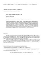
Fig. 7. The curve of composite waves Γ = W1 (UL
) ∪ L ∪ W1@ (UL ) defined by (4.18), and an intersection of Γ and the curve W2 (UR )
@
on the path W1 (UL
) that leads to a Riemann solution.

We now define
Γ = W1 UL@ ∪ L ∪ W1@ (UL ),

(4.18)

where UL@ , L and W1@ (UL ) are defined by (4.11), (4.13) and (4.17), respectively. Since the two end-points
of L corresponding to α = αR and α = αL coincide with the an end-point of W1 (UL@ ) and W1@ (UL ),
respectively, Γ is a (continuous) curve.
Any intersection point UM between the curve of the composite waves Γ and the backward curve of
2-waves W2 (UR ) could complete the Riemann solution by a 2-wave from UM to UR . The curves Γ and
W2 (UR ) in fact intersect whenever
ω1 UL@ ; 0 > ω2 (UR ; 0),

@
Φ2 UR , UL∗
< 0.

However, when UR ∈ G3 and the intersection point UM is located in the region u < us , the compatibility
condition
σ2 (UM , UR ) ≥ λ5 (UM )

(4.19)

must hold, in order for the 2-wave W2 (UM , UR ) to precede the 5-contact wave arriving at UM . As seen from
Proposition 3.2, there corresponds to any point U ∈ W1@ (UL ), u < us , a point U ∈ W2 (U ) ∩ G3 such that
σ2 U, U

= λ5 (U ).

Let Δ denote the set of these points U # , which form a curve in G3 :


M.D. Thanh / J. Math. Anal. Appl. 418 (2014) 569–594

Δ = U ∈ G3 : W2 (U ) ∩ W1@ (UL ) = U

,

591

(4.20)

where U is defined in Proposition 3.2 (part (b)), which satisfies
σ2 U, U

= λ5 (U ).

Geometrically, the condition (4.19) means that UR is located above or on the curve Δ.
Interestingly, whenever UL@# is located below the curve W2 (UR ) and UL#@ is located above it, the curve
W2 (UR ) intersects with all the three parts W1 (UL@ ), L, and W1@ (UL ). The Riemann problem then admits

three distinct solutions with different configurations. The above argument leads us to the following result
on the existence of Riemann solutions.
Theorem 4.1 (Existence for large data). Consider the case UL ∈ G1 ∪ C+ , αL ≤ αR . Assume that the
right-hand state UR ∈ G1 ∪ C ∪ G2 such that
ρ@
L

uR −

u@
L

<

ρR

p (y)
dy,
y

+
0

0

ρR

p (y)
dy,
y

uR − u@
L∗ >

(4.21)

ρ@
L∗
@
@
@
@
where UL@ = (ρ@
L , uL ) and UL∗ = (ρL∗ , uL∗ ) are defined by (4.11) and (4.16), respectively. The Riemann
problem for (1.1) admits a solution made of Lax shocks, rarefaction waves, and admissible contacts.

Remark 4.1. As indicated in the above argument, the result of Theorem 4.1 is still valid if the condition UR
is above G3 is replaced by a weaker condition that UR is above Δ defined by (4.20), see Fig. 7.
Proof. It is easy to see that the curve W1@ (UL ) defined by (4.17) can be parameterized by a function
u = u1@ (ρ). Furthermore, let us show that this function u1@ is decreasing. Indeed, if there were two states
U1 = (ρ1 , u1 ) and U2 = (ρ2 , u2 ) on the curve W1 (UL ), U1 is on a higher position than U2 such that
u1@ (ρ1 ) < u1@ (ρ2 ),
i.e., the state Υ (U1 , aL , aR ) is on a lower position than the state Υ (U2 , αL , αR ) on the curve W1@ (UL ). By
continuity, there would exist two states V1 , V2 ∈ W1 (UL ) ∩ G2 , V1 is on a higher position than V2 on W1 (UL )
such that
Υ (V2 , αL , αR ) = Υ (V1 , αL , αR ) := V0 ,
which is a contradiction, since there is a unique admissible 5-contact, which does not cross the resonant
surface, from V0 with the gas volume fraction αR to another state with the gas volume fraction αL .
Next, the first inequality in (4.21) can be re-written as
ω1 UL@ ; 0 > ω2 (UR ; 0),

(4.22)

where ω1 and ω2 are defined by (2.17), (2.18) and (3.5). The condition (4.22) means that the u-intercept
of the “increasing” curve W2 (UR ) (curve parameterized as an increasing function of the specific volume as


M.D. Thanh / J. Math. Anal. Appl. 418 (2014) 569–594

592

a function of the density) is below the one of the “decreasing” curve W1 (UL@ ) in the (ρ, u)-plane. The second
inequality of (4.21) can be re-written as
@
u@
L∗ < ω2 UR ; ρL∗ ,

or
@
Φ2 UR , UL∗
< 0,

(4.23)

@
where Φ2 is defined by (4.9). The condition (4.23) means that the end-point UL∗
of Γ is located below
the curve W2 (UR ) in the (ρ, u)-plane. The above argument implies that the two curves Γ and W2 (UR )
intersect. This leads us to a Riemann solution whose configuration can be described as follows. First, let
the two curves Γ and W2 (UR ) intersect on the path WL (UL@ ), where UL@ = Υ (UL , aL , aR ). Let

UM ∈ W1 UL@ ∩ W3 (UR ).
The solution is described by
W5 UL , UL@ ⊕ W1 UL@ , UM ⊕ W2 (UM , UR ).

(4.24)

Second, let the two curves Γ and W2 (UR ) intersect on the path L. Let
UM ∈ L ∩ W3 (UR ).
The solution has the form
W5 (UL , U1 ) ⊕ S1 (U1 , U2 ) ⊕ W5 (U2 , U3 ) ⊕ W2 (U3 , UR ),

(4.25)

where U1 = Υ (UL , αL , α), U2 = U1# , U3 = Υ (U2 , α, αR ) for some α ∈ [αL , αR ]. Third, let the two curves Γ
and W2 (UR ) intersect on the path W1@ (UL ) and let
UM ∈ W1@ (UL ) ∩ W3 (UR ).
The solution is described by
W1 (UL , UN ) ⊕ W1 (UN , UM ) ⊕ W2 (UM , UR ),
where UN = Υ (UM , αR , αL ).

(4.26)

✷

Theorem 4.2 (Uniqueness). Under the assumptions of Theorem 4.1, the Riemann problem for (1.1) admits
a unique solution if
min Φ2 (UR , U ) > 0,

U ∈L

or

max Φ2 (UR , U ) < 0,
U ∈L

(4.27)

where Φ2 is defined by (4.9). In particular, if UR , UL ∈ G1 such that
ρR

p (y)
dy < u@
L +
y

u s < uR −
0

ρ@
L

p (y)
dy,
y

(4.28)

0

@
where UL@ = (ρ@
L , uL ) is defined by (4.11), then the Riemann problem for (1.1) admits a unique solution of
the form (4.24).


M.D. Thanh / J. Math. Anal. Appl. 418 (2014) 569–594

593

Proof. The condition (4.27) implies that the curve W2 (UR ) may intersect with Γ exactly either on the path
W1 (UL@ ), or on the path W1@ (UL ). Note that the path L is always on one side of W2 (UR ). It is clear that
the curve W1 (UL@ ) can be parameterized in such a way that the velocity is given as decreasing function of
the density. This is also the case for the curve W1@ (UL ), see the proof of Theorem 4.1. The curve W2 (UR )
is given by an increasing function u = ω2 (UR ; ρ). Thus, it follows from Theorem 4.1 that the intersection of
W2 (UR ) and Γ contains exactly one point. The Riemann problem therefore admit a unique solution. This
establishes the first conclusion.
Next, the inequality on the left of (4.28) means that
ω2 (UR ; 0) > us ,
where ω2 is defined by (2.18). Since the slope of ω2 is larger than the one of C+ , the last inequality implies
that the curve W2 (UR ) remains in G1 . Therefore, the path L is located below W2 (UR ). In this case, W2 (UR )
intersects with Γ only on the path W1 (UL@ ). This yields the second conclusion. Theorem 4.2 is completely
proved. ✷
Acknowledgments
This research is funded by Vietnam National Foundation for Science and Technology Development
(NAFOSTED) under grant number 101.02-2013.14.
References
[1] L. Ambrosio, N. Fusco, D. Pallara, Functions of Bounded Variation and Free Discontinuity Problems, The Clarendon
Press, Oxford University Press, New York, 2000.
[2] A. Ambroso, C. Chalons, F. Coquel, T. Galié, Relaxation and numerical approximation of a two-fluid two-pressure diphasic

model, ESAIM M2AN Math. Model. Numer. Anal. 43 (2009) 1063–1097.
[3] N. Andrianov, G. Warnecke, The Riemann problem for the Baer–Nunziato model of two-phase flows, J. Comput. Phys.
195 (2004) 434–464.
[4] M.R. Baer, J.W. Nunziato, A two-phase mixture theory for the deflagration-to-detonation transition (DDT) in reactive
granular materials, Int. J. Multiph. Flow 12 (1986) 861–889.
[5] F. Bouchut, Nonlinear Stability of Finite Volume Methods for Hyperbolic Conservation Laws, and Well-Balanced Schemes
for Sources, Front. Math., Birkhäuser, 2004.
[6] J.B. Bzil, R. Menikoff, S.F. Son, A.K. Kapila, D.S. Steward, Two-phase modelling of a deflagration-to-detonation transition
in granular materials: a critical examination of modelling issues, Phys. Fluids 11 (1999) 378–402.
[7] G. Dal Maso, P.G. LeFloch, F. Murat, Definition and weak stability of nonconservative products, J. Math. Pures Appl.
74 (1995) 483–548.
[8] P. Goatin, P.G. LeFloch, The Riemann problem for a class of resonant nonlinear systems of balance laws, Ann. Inst. H.
Poincare Anal. Non Lineaire 21 (2004) 881–902.
[9] G. Hernández-Duenas, S. Karni, A hybrid algorithm for the Baer–Nunziato model using the Riemann invariants, J. Sci.
Comput. 45 (2010) 382–403.
[10] E. Isaacson, B. Temple, Nonlinear resonance in systems of conservation laws, SIAM J. Appl. Math. 52 (1992) 1260–1278.
[11] E. Isaacson, B. Temple, Convergence of the 2 × 2 Godunov method for a general resonant nonlinear balance law, SIAM J.
Appl. Math. 55 (1995) 625–640.
[12] B.L. Keyfitz, R. Sander, M. Sever, Lack of hyperbolicity in the two-fluid model for two-phase incompressible flow, Discrete
Contin. Dyn. Syst. Ser. B 3 (2003) 541–563.
[13] P.G. LeFloch, Entropy weak solutions to nonlinear hyperbolic systems under nonconservative form, Comm. Partial Differential Equations 13 (1988) 669–727.
[14] P.G. LeFloch, Shock waves for nonlinear hyperbolic systems in nonconservative form, Institute for Math. and Its Appl.,
Minneapolis, 1989, Preprint #593.
[15] P.G. LeFloch, M.D. Thanh, The Riemann problem for fluid flows in a nozzle with discontinuous cross-section, Commun.
Math. Sci. 1 (2003) 763–797.
[16] P.G. LeFloch, M.D. Thanh, The Riemann problem for shallow water equations with discontinuous topography, Commun.
Math. Sci. 5 (2007) 865–885.
[17] P.G. LeFloch, M.D. Thanh, A Godunov-type method for the shallow water equations with variable topography in the
resonant regime, J. Comput. Phys. 230 (2011) 7631–7660.
[18] D. Marchesin, P.J. Paes-Leme, A Riemann problem in gas dynamics with bifurcation. Hyperbolic partial differential

equations III, Comput. Math. Appl. (Part A) 12 (1986) 433–455.