DSpace at VNU: Homogenization of Rough Two-Dimensional Interfaces Separating Two Anisotropic Solids
Bạn đang xem bản rút gọn của tài liệu. Xem và tải ngay bản đầy đủ của tài liệu tại đây (4.62 MB, 8 trang )
Pham Chi
e-mail;
Do Xuan Tung
Faculty of Mathematics,
Mechanics and Informatics,
Hanoi University of Science,
334,
Nguyen Trai Street,
Thanh Xuan,
Hanoi 10000, Vietnam
Homogenization of Rough
Two-Dimensional Interfaces
Separating Two Anisotropie
Soiids
In this paper we have derived homogenized equations in explicit form of the linear
elasticity theory in a two-dimensional domain with an interface highly oscillating between two straight lines, by using the homogenization method. First, the homogenized
equation in the matrix form for generally anisotropic materials is obtained. Then, it is
written down in the component form for specific cases when the materials are orthotropic, monoclinic with the symmetry plane at X, =0 and X2 =0. Since these equations are
in explicit form, they are significant in practical applications. [DOI: 10.1115/1.4003722]
Keywords: homogenization, homogenized equations, very rough interfaces, anisotropic
materials
1
Introduction
Boundary-value problems in domains with rough boundaries or
interfaces appear in many fields of natural sciences and technology such as scattering of waves on rough boundaries [1-4]; transmission and reflection of waves on rough interfaces [5-7]; mechanical problems concerning the plates with densely spaced
stiffeners [8]; the flows over rough walls [9]; nearly circular hole,
inclusion problems in plane elasticity and thermoelasticily
[10-12]; and so on. When the amplitude (height) of the roughness
is much small in comparison with its period (see, for example,
Ref. [12]), the problems are usually analyzed by perturbation
methods [13]. When the amplitude is much large than its period,
i.e., the boundaries and interfaces are very rough (see, for instance, Refs. [14,15]), the homogenization method [16-18] is required, in which the very rough boundaries or interfaces are replaced with equivalent layers within which homogenized
equations hold (see Ref. [15]). The main aim of the homogenization of very rough boundaries or interfaces is to determine these
homogenized equations.
Nevard and Keller [15] examined the homogenization of very
rough three-dimensional interfaces separating two linear anisotropic solids. The authors have derived the homogenized equations, but these equations are still implicit. In particular, their coefficients are the solution of a boundary-value problem on the
periodic cell (called "cell problem"), which includes 27 partial
differential equations. This problem can, in general, only be
solved numerically. Recently, Vinh and Tung [19] considered the
homogenization of two-dimensional very rough interfaces separating two isotropic linear elastic solids, and they have derived the
explicit homogenized equations, by using the standard techniques
of the homogenization method along with the matrix formulation.
In this paper, following the procedure carried out in Ref. [19], we
have derived the explicit homogenized equation in the matrix
form for the case of generally anisotropic materials. Then, it is
written down in the component form for the specific cases when
the materials are orthotropic, and monoclinic with the symmetry
plane at X|=0 and X2=0. Since these equations are in explicit
Corresponding author.
Contributed by the Applied Mechanics Division of ASME for publication in the
JOURNAL OF APPI.IKD MKCHANICS. Manu.script received Augu.st 4. 2010; final manuscript received January 22, 2011; accepted manuscript posted February 28. 2011;
published online April 14, 2011. Assoc. Editor: Krishna Garikipati.
Journai of Appiied Mechanics
form, i.e., their coefficients are explicit functions of given material
and interface parameters, they are convenient in use. We also note
that homogenized equation (9.24) in Ref. [ 15] obtained by Nevard
and Keller is incorrect at least in the two-dimensional case (Remark 2).
Before going to Sec. 2, we recall once again the main point of
the homogenization of a very rough interface oscillating between
two straight lines and separating two elastic solids. Due to great
difficulties caused by its rapid oscillation, the interface (or the
composite material layer containing the interface) is replaced with
an equivalent elastic plane layer. Then the actual problem is replaced with the problem of two dissimilar elastic half-spaces separated by an elastic plane layer with homogenized propenies. This
material layer is governed by the homogenized equations, which
need to be determined.
2
Basic Equations in Matrix Form
Consider a linear elastic ix)dy that occupies two-dimensionai
domains fl* and fl" of the plane X\Xy, their interface L oscillates
between two straight lines Xj=-A (i4>0) and X3=0, and is expressed by the equation X3=/4/i(X|/\) ( \ > 0 ) , where h{y) {y
= X | / \ ) is a periodic function of period 1 whose maximum and
minimum values are 0 and - 1 , respectively, as described in Fig.
1. Suppose that in the domain 0 < X | < \ , i.e., 0 < v < l , any
straight line X3=X^=const (-/1
and ÎÏ-.
Suppose that the body is made of a generally anisotropic material. Since the inplane deformations cannot be decoupled from the
antiplane deformations for this case (see Ref. [20]), we are thus
concemed with the generalized plane strain, for which the displacement components «,, «2, and M3 are all nonzero and
(=1,2,3
(1)
where / is the time. For this case, the stresses cr,y are related to the
displacement gradients u¡j by [20]
Copyright © 2011 by ASiME
{j
-^ M3 )
JULY2011, Vol. 78 / 041014-1
Fig. 1 Two-dimensional domains û* and n~ have a very rough
interface Í. expressed by equation X3=Ah(X^I\) = Ah{y), where
h(,y) is a periodic function with period 1, and its maximum and
minimum values are 0 and - 1 , respectively. The curve L oscillates between the straight lines ^3=0 and X3=-A.
Fig. 2 The interface L in the x^Xstraction vector and the displacement vector must be satisfied. Thus
we have
[(A,,U.I + A|3U,3)Ai, + (A31U.1 -I- A33U.3)AÍ3]i = 0,
[U]L = 0
(8)
O-33 =
(2)
0^23 = Cl4«l.l + C34«3.3 + i^44"2.3 + i'45("l.
where A'^ is the X^^-component of the unit normal to the curve L,
and we introduce the notation [. ]¿, defined such as
on L
0-3: = C|5"l.l + C.35"3.3 + C45"2.3 + C.«(«1.
where commas indicate differentiation with respect to the spatial
variables X,, and c¡j are material constants,. Equations of motion
are [20]
O'l3.3+/l=P"l
S | = A | | U ,+A,3U3,
for
for
(4)
(10)
Xi = Xi/A
(11)
Then, in the j:|A:3-plane, the curve L (see Fig. 2) is expressed by
x^ = h{y),
in which / i , /2, and f-^ are the components of the body force, p is
the mass density, and a superposed dot signifies differentiation
with respect to time t. The material constants i^ and the mass
density p are defined as
S3 = A3,U,i+A33U3
Now we introduce the new (dimensionless) variables
;c, =X,/A,
(3)
(9)
Note that the traction vectors on the planes perpendicular to the
X|-axis
and X3-axis,
2i=[o-ii (7|2 0-13]^ and ^ 3
=[fi3 i^23 C33 ]^, namely, are determined by
y = .ï|/e(=X,/X)
(12)
where h{y) is a periodic function with period 1, as said above. In
terms of these new variables, Eq. (5) becomes
{\,„u,,)_, + f = ßü
(13)
where commas indicate differentiation with respect to the variables x¡, and
F = A^F,
p = A^p
(14)
where c¡j.^, c¡j_, p.^, and p_ are constant. Introducing Eq. (2) into
equations of motion (3) leads to a sy.stem of equations for the Similarly, continuity condition (8) now takes the form
displacement components whose matrix form is
[(A||U| -I-A|3U3)«| +(A3|U| + A33U 3)«3]i, = 0, [u]i = O
(15)
in which u = [uiU2U2,Y and 'P=[fff2fiiY< the symbol T indicates where «^ is the jc^-component of the unit normal to the curve L (in
the transpose of a matrix, the indices h and k take the values 1 and the ;C|X3-plane). Note that
3, and 3 X 3-matrices A/,^ are given by
Ni:N^=n^:nf = \:-f-^h'(y)
(16)
Taking into account of the second equality of Eq. (16), continuity
condition (15) can be written as
(6)
(17)
3 Explicit Homogenized Equation in Matrix Eorm
(7)
Following Bensoussan et al. [16], Sanchez-Palencia [17], Bakhvalov and Panasenko [18], and Köhler et al. [14] we suppose
that u{Xi,xi,,t,e) = l]{x[,y,X2,t,e), and we express U as follows
[19]:
U = V -f- e(N'V + N"V.| + N'-'V.3) + e^(N^V + N^'V,, + N " V . 3
are defined by Eq. (6) in which C;, are replaced
where
with c^j icjj). Since the matrix (c,;)6x6 's positive definite [20], it
follows that All is invertible. Suppose that il* and il' are perfectly welded to each other along L. then the continuity for the
041014-2 / Vol. 78, JULY 2011
+
N2"V.||
+ '-N2'yi3-i-N-"V..3.3)
+ ^y^
O(f'))
(18)
'^'^
".n +
"1 *.i3 + i^ ^.^il +
where V = V ( . Ï | , . Ï 3 , / ) (being independent of >), N', N " , N ' \ N^,
N^', N^^, N^", N^'^ and N^-^' are 3X3-matrix valued functions
Transactions of the ASME
of y and x^ (not depending on A:,, t), and they are y-periodic with
period 1. The matrix valued functions N'
, N-^" are determined
so that Eq. (13) and continuity conditions (17) are satisfied. Since
y=x¡/e, we have
u , = U , + e-'U,
[ A | , N f + A,3Ni']i = 0 at y„>.2
Finally, by integrating Eq. (25) along the line jC3=const, -1
(26)-(31), we obtain the homogenized equation, namely.
(19)
We now follow the same procedure as one carried out in Ref. [19].
First, introducing Eq. (18) into Eqs. (13), (17),, and (H),, and
taking into account Eq. (19) yield equations that we call equations
(fl), (É'2), and (63), respectively. In order to make the coefficients
of e"' of equations (i'|) and ((?2), and the coefficients of e of
equation (^3) zero, the functions N', N", and N " are chosen so
that
+ [{(A33) +
-1
0<.v
A^t_V.„, + F_ = p_V, ;c3 < - 1
(33)
y it y,,
(20)
]i = O at ^„^2;
(32)
For the domains X3 > 0 and ;iC3 < - 1 , we have
AM+V,^;, + F., = p^V, .13 > 0 ;
[ A „ N ^ , = O,
(31)
N'(O) =
On the lines .1:3=0 and Ar3=-1 the continuity conditions are required and they are
7;)-'V,, + {(A33)
(21)
N"(O) = N"(1)
= O at
(34)
and
[V]¿. = 0,
(22)
0, at ^1,^2;
N'-^(O)
where E is the identity 3x3-matrix, and V| and y2 (O<>'|<>'2
< 1) are two roots in the interval (0,1) of the equation h{y)=x^ for
y, in which x^ belongs to the interval (-1,0). From Eqs.
(20)-(22), it is not difficult to verify that
¿* is lines X3 = 0,
=- 1
Note that continuity condition (34), is originated from the request
[23],.=0 on the lines ^3=0 and X3=--4, where by X^' (*= 1,3) we
denote the leading term of 2^.
In terms of the variables Xi¡, Eqs. (32)-(34) take the form
N]y = 0,<A3,(E -h N^)) = (A3,A7;)(A7;>-'
(F)-
-
(35)
(23)
-A
(36)
where
(37)
(24)
(<P>
Jo
Second, equating to zero the coefficient e" of equation {e¡) and
taking into account the fact N'y=O lead to
FA N^ A N ' I V TA Í N ' N ^ ' I A N " 1 V TA l v "
" •'
'^ •' '^
"
•>•
" •'•'•^ •' '- " •>'
+ A|3(N'+N3^)]j,V_3 + {[A,,(N" + N^^")]^ + A||(E
+ A,,N,\'}V,,3 + [A, , N f + A,3N'-1,V.33 + (A33V,3).3
-h [A3,(E -h N,y )V,| + A3,N;;V,3],3 + F - pV = 0
at
[V]£. = 0, L' is lines ^3 = 0,
Equation (35) is desired homogenized equation whose coefficients
are explicit functions of material and interface parameters. This
equation defines the solution \{X¡,Xi,,t), which is the leading
term of u{X¡,X^,t,e) in expansion (18); thus it is the limit of
u(X| ,Xj,,t,e) when e tends to zero.
Remark I.
./
(i)
It is not difficult to verify that
;
.^ ''
(25)
In order to make the coefficients of e" of equation (¿'2) zero we
take (noting that N'^,=O)
= O
and
(26)
at
^
'
at
X(A7,')-'V., -h [(A33) +
(38)
and Eq. (35) is of the form
...
.,
(39)
(ii) When the interface L is of tooth-comb type (see Fig, 3),
Eq, (35) is simplified to
(28)
(29)
(30)
Journal of Applied Mechanics
+ (F)-(p)V>=0
where
(40)
JULY 2011, Vol. 78 / 041014-3
Keller's notations) are constants with different values in fl^ and
n~. From this fact, it can be shown that the correct homogenized
equation for the two-dimensional case is Eq. (9.24) in Ref. [15], in
which M„„„ = 0 (the right-hand side of Eq. (9.24) in Ref. [15]
must be zero).
a+b
4 Special Cases: Homogenized Equations in Component Form
4.1 Monoclinic Materials With the Symmetric Plane X|
=0. For the monoclinic materials with the symmetry plane X|
=0, we have [20]
C,5 = Í:^ = 0,
;fc= 1,2,3,4
(42)
Introducing Eq. (42) into Eq. (6) yields
Fig. 3 The tooth-comb interface L. L^:X^=
0), L3:X3=0(0£Xisa), and
0
A,,=
0
0
0
C56
-
0
i'l4
^13
C56
0
0
.'•55
0
0
"'•55
0
0
0
644
C34
0
C34
''33
A,3 =
C56
(43)
0
(41)
(
a+b
A,,=
Note that all coefficients of Eq. (40) are constant.
Remark 2. For the two-dimensional case, from Eqs. (9.12) and
(9.13) in Ref. [15], one can show that Cyt^óty^tmn (in Nevard and
f|4
0
0
.''13
0
0
.
A33 =
On the use of Eq. (43), we can write Eqs. (35)-(37) in the component form as
' • '.
, I + C55+V1 33 -I- (C56+ -I- C|4+)^2,13 + (C55+ + C13J V3J3 - 1 - / , ^ = p+V>,, X3 > 0
11 + C44.^V2,33 + (c¡f,+ + C14+) V,.,., + C56+V3 ,, -I- C34+V3 33 + fj^ = P+V2, X3 > 0
Cs5+yjA\ + (C55+ + C13JV'|,|3 + C¡(^V2_u + C34+V2,33 + / 3 ^ = p^Vj,
(44)
X3 > 0
cii
J»
Cll/
\
'•'.
Cu
•'-
J.
/ J
J,3
(45)
f|3
£•11/
*ll(..).i,A-/\-/-\
-^1.33 + (C55.- + «•|4-)
'1,1
J.3
'-(^;iK,
X3 < - A
^2. X3 < - /
(46)
V'3- X3 <-
041014-4 / Vol. 78, JULY 2011
Transactions of the ASME
V„ V2
are continuous on X3 = - A ,
X3
^cl„
(47)
8{c,,/S>{c^S){c,^S)
Note that when il* and iiir are made of the same mal
material, ¿-¡j
=c¡j; thus systems (44)-(46) are identical to each other.
other
where
3 + ^56^2 1
4.2 Monoclinie Materials With the Symmetrie Plane X2
the mon
monoclinie materials with the symmetry plane Xo
~^- ^°^r ^^^
=0, We •have [20]
(48)
Substituting Eq. (50) into Eq. (6) yields
||
A,,=
0
|
Cl5
0
C,3
0
C66
0
0
C4,
0
C|5
0
C55
.C55
0
f,5
15
0
C55
C55
0
0
C45
0
0
C44
0
^Cl3
0
[f35
0
(•33_
(51)
A,,=
and
ij = 5,6
, .„^ '
,
C-35J
A33=
On the use of Eq. (51 ), we can write Eqs. (35)-(37) in the component form as
J
I + V'i,, + 2C|5^V| ,3
= p^.V|, X 3 > 0
3,|,
= p,V>3, X 3 > 0
-35+V, 33 -1- c¡¡^V¡j, -1- 2035.^^3
5+V|,n -I- (f55+ + c n
(52)
2^ = P+V'2. X3 > 0
V,,,3 + [(c, ,(
.3] 3
(53)
C, | _ V , . | ,
5_V3,,,
ClS-V'l.l 1 + (C55- -H C13
^b
Vi, V3,
a-23, 033 are continuous on X3 = - j
=0
5_V3 33 + f, = p_V„ X3 <
-^ C55_V3
,,
,,3 -I- C33_V3 33 -I-/3 = p_V>3, X3 <
„V*
(54)
X3
(55)
where
in which
V3,,) -h (C|5(a)
c¡j = {c¡j/d}/d, i,j= 1,5, d =
= (C, 1(0) + C|5<è))V,., -I- (C,5(a
(56)
Journal of Applied Mechanics
(57)
JULY 2011, Vol. 78 / 041014-5
= 1,2,3,
- ((
ö, =
(59)
= 1,2,3,
Note that when the materials of ü,* and fl" are the same, we have
i,j=\,5,
(58)
a = c 13, ¿ = C35, a , = C33
From Eqs. (50) and (59) one can see that an orthotropic material is
a monoclinic material with the symmetry plane X2=0 subjected to
the constraints 0*5=0, ¿ = 1 , 2 , 3 , C46=0. Introducing the facts
Cki=O, k=l,2,3,
C46=0 into Eqs. (52)-(56) and taking into account Eq. (57) yield the homogenized equations for the orlholropic case, namely.
Systems (52)-(54) thus coincide with each other. From Eqs.
(52)-(54) it is clear that «i and M3 decoupled from «2. In other
words, the inplane deformations are decoupled from the antiplane
deformations for this case (see also Ref. [20]).
(Cl3+ + C55+)V, ,3 + C55+V3_,, + C33+V3,33 + / 3 ^ = P+V3, X3 > 0
C66..V'2,,, + C44^V2.33 -H/2^ = P+V2, X3 > 0
4.3 The Case of Orthotropic Materials. For orthotropic materials we have [20]
- ;
v,,3
£•55/
0
l.ll + C55+V1.33 +
(60)
+ K - ; V,,
J.3
L\C55/
'3.13
J.3
-1
/V/
— ; V 3.11
,,,
(61)
1 \-7-.3^^ '^'
'•11/
\ c i i
- A
+ £'55-)
33_V3,33 -l-/3_ = p.V,, X3 < - A
(C,3. -I- C55.)V,,,3
V,, V2, V3, (T"3, fr23 (7-33 continuous on X3 = -
(63)
where
(62)
clinic with the symmetry plane at X,=0 and X2=0, we have arrived at the homogenized equations in the component form. Since
the obtained equations are in explicit form, they are good tools for
investigating various practical problems.
Acknowledgment
The work was supported by the Vietnam National Foundation
For Science and Technology Development (NAFOSTED) under
Grant No. 107.02-2010.07.
(64)
References
From Eqs. (60)-(62) and (64), it is clear that the inplane deformations are also decoupled from the antiplane deformations for
orthotropic materials. Note that Eqs. (60)-(62) and (64) can also
be derived from homogenized equations (44)-(46) and (48) for
the monoclinic materials with the symmetry plane X|=0, by vanishing the constants Q4(Â:=1 ,2,3) and c¡(,.
5
Conclusions
In this paper is investigated the homogenization of a twodimensional interface that separates two anisotropic elastic solids
and highly oscillates between two straight lines. For generally
anisotropic materials we have obtained the homogenized equation
in the matrix form. When the materials are orthotropic, and mono041014-6 / Vol. 78, JULY 2011
[I] Zaki. K. A., and Neureuther. A. R.. 1971. "Scattering From a Perfeclly Conducting Surface With a Sinusoidal Height Profile; TE Polarization," IEEE
Trans. Antennas Propag.. 19, pp. 208-214.
[2] Waterman, P. C , 1975, "Scattering by Periodic Surfaces," J. Acoust. Soc. Am.,
57. pp. 791-802.
[3] Belyaev. A. G., Mikheev. A. G.. and Shamaev. A. S.. 1992, "Plane Wave
Diffraction by a Rapidly Oscillating Surface." Comput. Math. Math. Phys..
32. pp. 1121-11.«.
[4] Bao. G., and Bonnetier, E., 2001, "Optimal Design of Periodic Diffractive
Structures." Appl. Math. Optim., 43, pp. 103-116.
[5] Talbot. J. R. S.. Titchener. J. B.. and Willis. J. R.. 1990. "The Reflection of
Electromagnetic Waves From Very Rough Interfaces," Wave Motion. 12. pp.
245-260.
[6] Singh. S. S.. and Tomar, S. K., 2007, "Quasi-P-Waves at a Comigated Interface Between Two Dissimilar Monoclinic Elastic Half-Spaces," Int. J. Solids
Struct.. 44. pp. 197-228.
[7] Singh. S. S.. and Tomar, S. K.. 2008, "qP-Wave at a Corrugated Interface
Between Two Dissimilar Pre-Stressed Elastic Half-Spaces." J. Sound Vib..
317. pp. 687-708.
Transactions of the ASME
[8] Cheng, K. T.. and Olhoff, N.. 1981, "An Investigation Concerning Optimal
Design of Solid Elastic Plates," Int. J. Solids Strucl., 17, pp. 795-810.
[9] Achdou. Y.. Pironneau. O.. and Valentin. F.. 1998. "Effective Boundary Conditions for Laminar Flows Over Rough Boundaries." J. C'omput. Phys.. 147.
pp. 187-218.
[10] Givoli. D.. and Elishakoff. I., 1992, "Stress Coneentralion at a Nearly Circular
Hole With Uncertain Irregularities," ASME J. Appl. Mech., 59, pp. S65-S7I.
[II] Wang. C.-H.. and Chao. C.-K.. 2002. "On Pertuhation Solutions of Nearly
Circular Inclusion Problems in Plane Thentioela.sticity." ASME J. Appl.
Mech.. 69. pp. 36-44.
[12] Ekneligoda, T. C . and Zimmermam, R. W.. 2(X)8. "Boundary Pertubation Solution for Nearly Circular Holes and Rigid Inclusions in an Infinite Elastic
Medium." ASME J. Appl. Mech.. 75. p. 011015.
[13] van Dyke. M.. 1975. Pertubation Methods in Fluid Mechanics, Parabolie,
Stanford, CA.
[14] Köhler. W.. Papanicolaou. G. C , and Varadhan, S.. 1981 "Boundary and Interface Problems in Regions With Very Rough Boundaries." Multiple Scatter-
I
V
ing and Waves in Random Media, P. Chow, W. Köhler, and G. Papanicolaou,
eds., North-Holland. Amsterdam, pp. 165-197.
[15] Nevard. J.. and Keller. J. B.. 1997. "Homogenization of Rough Boundaries and
Interfaces," SIAM J. Appl. Math.. 57. pp. 1660-1686.
[16] Bensoussan. A.. Lions. J. B.. and Papanicolaou, J.. 1978. Asymptotic Analysb
for Periodic Structures, North-Holland. Amsterdam.
[17] Sanchez-Palencia. E., 1980. Nonhomogeneous Media and Vibration Theory
(Lecture Notes in Physics. Vol. 127). Springer-Verlag. Heidelberg.
[18] Bakhvalov, N., and Panasenko. G.. 1989. Homogenisation: Averaging of Processes in Periodic Media: Mathematical Problems of the Mechanics of Composite Materiah, Kluwer. Dordrecht.
[19] Vinh, P. C , and Tung, D. X.. 2010. "Homogenized Equations of the Linear
Elasticity in Two-Dimensional Domains With Very Rough Interfaces." Mech.
Res. Commun., 37. pp. 285-288.
[20] Ting, T. C. T . 1996. Anisotropic Elasticity: Theory and Applications. Oxford
University Press, New York.
1
'•' . ••
Journal of Appiied Mechanics
JULY 2011, Vol. 78 / 041014-7
Copyright of Journal of Applied Mechanics is the property of American Society of Mechanical Engineers and
its content may not be copied or emailed to multiple sites or posted to a listserv without the copyright holder's
express written permission. However, users may print, download, or email articles for individual use.