DSpace at VNU: The finite Hartley new convolutions and solvability of the integral equations with Toeplitz plus Hankel kernels
Bạn đang xem bản rút gọn của tài liệu. Xem và tải ngay bản đầy đủ của tài liệu tại đây (268.4 KB, 13 trang )
J. Math. Anal. Appl. 397 (2013) 537–549
Contents lists available at SciVerse ScienceDirect
Journal of Mathematical Analysis and
Applications
journal homepage: www.elsevier.com/locate/jmaa
The finite Hartley new convolutions and solvability of the integral
equations with Toeplitz plus Hankel kernels
Pham Ky Anh a , Nguyen Minh Tuan b,∗ , Phan Duc Tuan c
a
Department of Comput. and Appl. Math., College of Science, Vietnam National University, 334 Nguyen Trai str., Hanoi, Viet Nam
b
Department of Math., College of Education, Viet Nam National University, G7 build., 144 Xuan Thuy rd., Cau Giay dist., Ha Noi, Viet Nam
c
Department of Math., Pedagogical College, University of Da Nang, 459 Ton Duc Thang str., Da Nang city, Viet Nam
article
info
Article history:
Received 20 March 2012
Available online 9 August 2012
Submitted by G. Chen
Keywords:
Generalized convolution
Fourier series
Hartley series
Integral equation of convolution type
abstract
The main aim of this work is to consider integral equations of convolution type with
the Toeplitz plus Hankel kernels firstly posed by Tsitsiklis and Levy (1981) [11]. By
constructing eight new generalized convolutions for the finite Hartley transforms we
obtain a necessary and sufficient condition for the solvability and unique explicit
L2 -solution of those equations. Thanks to this convolution approach the solvability
condition obtained here is remarkably different from those in Tsitsiklis and Levy (1981) [11]
and in other papers.
© 2012 Elsevier Inc. All rights reserved.
1. Introduction
Consider the integral equation of the form
λϕ(x) +
b
[p(x − u) + q(x + u)] ϕ(u)du = f (x),
(1.1)
a
where λ ∈ C, −∞ ≤ a < b ≤ +∞, and K (x, u) := p(x − u) + q(x + u) is the kernel of the equation. Eq. (1.1) with a Toeplitz
p(x − u) or Hankel q(x + u) kernel attracts attention of many authors as they have practical applications in such diverse
fields as scattering theory, fluid dynamics, linear filtering theory, and inverse scattering problems in quantum-mechanics,
problems in radiative wave transmission, and further applications in Medicine and Biology (see [1–11]). The historical
development concerning Eq. (1.1) as well as its applications can be found in the above-mentioned works. In particular,
Eq. (1.1) has been carefully studied when K (x, u) is a Toeplitz p(x − u), Hankel kernel q(x + u), or K (x, u) = p(x − u)+ p(x + u),
i.e. the Toeplitz and Hankel kernels are generated by the same function p.
In 1981, Tsitsiklis and Levy [11] considered Eq. (1.1) with general Toeplitz plus Hankel kernels p(x − u) + q(x + u).
Toeplitz plus Hankel kernels also appear in the study of a circular punch penetrating a finitely thick elastic layer resting on
a rigid foundation, in that of atmospheric scattering, and in rarefied gas dynamics. Moreover, Eq. (1.1) is a generalization
of Levinson equations considered by Chanda and Sabatier [4] for the Toeplitz case and of that studied by Agranovich and
Marchenko [1] for the Hankel kernel.
Integral operators defined by the Toeplitz plus Hankel kernels are closely related to Wiener–Hopf plus Hankel type
operators that are the vigorously studied objects. With respect to both numerical and theoretical investigations there have
been many efforts, implicit or explicit, to study Eq. (1.1) in different spaces of functions. For example, by assuming that the
∗
Corresponding author.
E-mail addresses: (P.K. Anh), (N.M. Tuan), (P.D. Tuan).
0022-247X/$ – see front matter © 2012 Elsevier Inc. All rights reserved.
doi:10.1016/j.jmaa.2012.07.041
538
P.K. Anh et al. / J. Math. Anal. Appl. 397 (2013) 537–549
functions p, q are twice continuously differentiable over all R, the work [11] investigated some operator characteristics and
gave numerical solutions to Eq. (1.1). Under an assumption that the kernel K (x, u) is continuously differentiable in each of
variables x and u, Levinson reduced the problem to an appealing set of first order partial differential equations that admit
a recursive fast numerical solution and have been of particular use in the field of fast signal processing (see [3,12,11] and
references therein). Feldman et al. [13] provided a sufficient and necessary condition via partial indices for the invertibility
of the Toeplitz integral operator (without Hankel term) in the space of Lebesgue integrable functions on finite intervals. In
recent times, the papers [14–18] dealing with the cases of infinite domains of integration have been published.
Our study of Eq. (1.1) is motivated by continuous efforts of those studies as well as a sufficiently long list of abovementioned materials.
The aim of this paper is to study the solvability of the equation by a finite convolution approach. Our idea is constructing
convolutions for the Hartley transforms and reducing the initial integral equation to systems of two linear algebraic
equations. By determining solutions of those systems of equations, we obtain the L2 -solution which is an explicit Hartley
series. Thus, instead of the smoothness assumption for the kernel functions p and q, widely used in other works, we need
only their Lebesgue integrability and 2π -periodicity.
The paper is divided into three sections and organized as follows.
In Section 2.1 of Section 2, the known notions of the finite Fourier sine, cosine transforms and that of the finite Hartley
transforms are recalled, and some preparing lemmas related to the finite Hartley transforms are proved. In Section 2.2, we
construct eight new generalized convolutions for the finite Hartley transforms, and prove the main theorem with a mind
that the obtained generalized convolutions could be useful for other applications such as digital filtering, etc. Besides, it is
proved that, the Riemann integrability, 2π -periodicity and boundedness of only function f are sufficient for ensuring the
continuity of the convolution functions defined by (2.10)–(2.13), and (2.19)–(2.22).
Section 3 deals with the application involved in studying Eq. (1.1) which is our main interest. In Theorem 3.1, by assuming
that the functions p and q are 2π -periodic and square-integrable on [0, 2π ] we obtain a necessary and sufficient condition for
the solvability of Eq. (1.1) and its explicit solution is given by the Hartley series. It should be emphasized that the condition
in Theorem 3.1 is remarkably different from those in other papers (cf. [1,4,13,11]). Furthermore, we show the fact that
classical partial-differential equations on finite domains (for example, that are the elliptic, hyperbolic, or parabolic types)
can be solved effectively by using the Hartley transform and their convolutions.
2. Hartley transforms and their convolutions
2.1. Hartley transforms
We now begin with the precise definition of the Fourier series of a function. Write N := {0, 1, 2, 3, . . .}.
Definition 2.1 (See [19,20]). (a) Let f be a Lebesgue integrable function on a finite interval [0, 2π]. The finite Fourier cosine,
sine transforms of f are defined respectively as
Fc {f (x)}(n) =
Fs {f (x)}(n) =
π
1
2π
1
f (x) cos(nx)dx := f˜c (n),
n ∈ N,
(2.2)
f (x) sin(nx)dx := f˜s (n),
n ∈ N.
(2.3)
0
2π
π
0
(b) The infinite sum
(Ff )(x) :=
f˜c (0)
2
+
∞
f˜c (n) cos(nx) + f˜s (n) sin(nx)
(2.4)
n =1
is called the Fourier series of f on [0, 2π ] where f˜c (n), f˜s (n) are the Fourier coefficients of f .
At this point, we do not say anything about the convergence of series (2.4). Namely, there exists a function f ∈ L1 [0, 2π ]
such that its series (2.4) diverses at every x ∈ [0, 2π ]. However, if 1 < p < +∞ and if f ∈ Lp [0, 2π], then its series (2.4)
converges in mean (Lp -norm) to a function in Lp [0, 2π]. In the framework of this paper, only two spaces L1 [0, 2π ], L2 [0, 2π ]
are concerned.
Series (2.4) may be rewritten as follows
(Ff )(x) =
f˜c (0) + f˜s (0)
2
+
∞
f˜c (n) + f˜s (n)
n=1
2
[cos(nx) + sin(nx)] +
f˜c (n) − f˜s (n)
2
[cos(nx) − sin(nx)] .
The representation in the form (2.5) suggests us to define the finite Hartley transforms as follows.
(2.5)
P.K. Anh et al. / J. Math. Anal. Appl. 397 (2013) 537–549
539
Definition 2.2 (Finite Hartley Transforms, See Also [21,22]). (a) Let f be a Lebesgue integrable function on [0, 2π ]. The finite
Hartley transforms of f are defined by
2π
f (x)cas(nx)dx := f˜1 (n),
n ∈ N,
0
2π
1
H2 {f (x)}(n) =
2π
1
H1 {f (x)}(n) =
2π
(2.6)
f (x)cas(−nx)dx := f˜2 (n),
n ∈ N,
0
where the integral kernel, known as the cosine-and-sine or cas function, is defined as cas x := cos x + sin x.
(b) The infinite sum
(Hf )(x) := f˜1 (0) +
∞
f˜1 (n)cas(nx) + f˜2 (n)cas(−nx)
(2.7)
n =1
is called Hartley series of f on [0, 2π]. According to the above-mentioned convergence of (2.4) we can see that if f ∈
L2 [0, 2π ], then the right-hand side of (2.7) defines a function in space L2 [0, 2π].
We call f˜1 (n), f˜2 (n) the n-th Hartley coefficients of f corresponding to H1 , H2 , respectively. It is easily seen that for every
n ∈ N,
f˜1 (−n) = f˜2 (n),
and H1 {f (−x)}(n) = H2 {f (x)}(n),
1
1
(f˜c (n) + f˜s (n)),
f˜2 (n) = (f˜c (n) − f˜s (n)).
2
2
Theorem 2.1 below is an immediate consequence of the known results in Fourier analysis (see [20]).
f˜1 (n) =
(2.8)
(2.9)
Theorem 2.1. The set of functions
√
√
√
1/ 2π ; cas(nx)/ 2π ; cas(−nx)/ 2π : n ≥ 1
is an orthonormal basis of the Hilbert space L2 [0, 2π], and the following identities yield:
2π
1
2π
1
cas m(x + u)cas(nu)du = δmn cos nx,
0
2π
2π
cas m(x − u)cas(nu)du = δmn sin nx,
0
where δmn is the Kronecker delta.
The Hartley transforms H1 and H1 also have the uniqueness theorem and the Riemann–Lebesgue lemma. Namely, if
f ∈ L1 [0, 2π] with f˜1 (n) = f˜2 (n) = 0 for all n ∈ N, then f = 0; and if f ∈ L1 [0, 2π ], then
2π
lim
n→∞
cas(nx)f (x)dx = 0.
0
2.2. Convolutions
In general, Fourier coefficients of the product of two functions fg are not the product of the Fourier coefficients of f and
g. The notion of convolution of two functions is a nice idea focusing on the so-called factorization identity which plays a
fundamental role in Fourier analysis; namely, factorization identity of convolution says that the Fourier coefficients of f ∗ g
are the product of the Fourier coefficients of f and g. Finite Fourier convolution appears naturally not only in the context of
Fourier series but also serves more generally in the analysis of functions in other settings (see [19,20,23–25]).
Let ∥f ∥1 denote the norm of a function f in L1 [0, 2π ].
Theorem 2.2 (Convolution Theorem). Suppose that the function f defined on R is 2π -periodic. If f , g are Lebesgue integrable
on [0, 2π ], then each of integral transforms (2.10)–(2.13) below defines a generalized Hartley convolution followed by its norm
inequality and factorization identity:
(f ∗ g )(x) =
H1
1
4π
2π
∥f ∗ g ∥1 ≤ ∥f ∥1 ∥g ∥1 ;
H1
[f (x + u) + f (x − u) + f (−x + u) − f (−x − u)] g (u)du,
0
H1 {(f ∗ g )(x)}(n) = f˜1 (n)˜g1 (n).
H1
(2.10)
540
P.K. Anh et al. / J. Math. Anal. Appl. 397 (2013) 537–549
(f
∥f
(f
∥f
(f
∥f
∗
H1 ,H2 ,H2
g )(x) =
2π
1
4π
∗
g ∥1 ≤ ∥f ∥1 ∥g ∥1 ;
∗
g )(x) =
H1 ,H2 ,H2
H1 ,H2 ,H1
2π
1
4π
g ∥1 ≤ ∥f ∥1 ∥g ∥1 ;
∗
g )(x) =
H1 ,H1 ,H2
∗
H1 ,H1 ,H2
(2.11)
H1 {(f
∗
H1 ,H2 ,H2
g )(x)}(n) = f˜2 (n)˜g2 (n).
[−f (x + u) + f (x − u) + f (−x + u) + f (−x − u)] g (u)du,
(2.12)
0
∗
H1 ,H2 ,H1
[f (x + u) − f (x − u) + f (−x + u) + f (−x − u)] g (u)du,
0
2π
1
4π
H1 {(f
∗
H1 ,H2 ,H1
g )(x)}(n) = f˜2 (n)˜g1 (n).
[f (x + u) + f (x − u) − f (−x + u) + f (−x − u)] g (u)du,
(2.13)
0
g ∥1 ≤ ∥f ∥1 ∥g ∥1 ;
H1 {(f
∗
H1 ,H1 ,H2
g )(x)}(n) = f˜1 (n)˜g2 (n).
Moreover, if f , g are Riemann integrable and bounded on [0, 2π ], then the functions defined by the integrals on the right-handside of (2.10)–(2.13) are continuous.
To prove Theorem 2.2 we need the following lemmas.
Lemma 2.1. Let f be a 2π -periodic function. Assume that f is Lebesgue integrable on [0, 2π ]. The following identities hold for
any u ∈ [0, 2π ] and for every n ∈ N:
H1 {f (x + u) + f (x − u) + f (−x + u) − f (−x − u)}(n) = 2f˜1 (n)cas(nu),
(2.14)
H2 {f (x − u) + f (−x + u) + f (−x − u) − f (x + u)}(n) = 2f˜2 (n)cas(nu).
(2.15)
Proof. Let us first prove (2.14). Due to the assumptions, f is integrable on every finite interval [a, a + 2π ]. We have
2f˜1 (n)cas(nu) = 2cas(nu)
=
=
=
1
2π
π
2π
1
2π
f (x)cas(nx)dx
0
f (x)[cos(nu) cos(nx) + cos(nu) sin(nx) + sin(nu) cos(nx) + sin(nu) sin(nx)]dx
0
1
2π
f (x)[2 cos n(x − u) + 2 sin n(x + u)]dx
0
1
2π
2π
2π
f (x)[cas n(x − u) + cas n(−x + u) + cas n(x + u) − cas n(−x − u)]dx,
0
which is, by putting x − u = t , −x + u = t , x + u = t and −x − u = t,
=
2π
−
2π −u
1
f (t + u)cas(nt )dt +
−u
2π
2π
−2π+u
f (−t + u)cas(nt )dt +
1
2π
2π+u
f (t − u)cas(nt )dt
+u
−u
1
+u
1
−2π−u
f (−t − u)cas(nt )dt .
As the inner integral functions are 2π -periodic with respect to corresponding to variable t, the limits of integration can be
replaced with limits from 0 to 2π . Therefore,
2f˜1 (n)cas(nu) =
2π
+
=
1
2π
0
1
2π
0
2π
1
2π
f (t + u)cas(nt )dt +
2π
2π
f (t − u)dtcas(nt ) −
2π
1
f (−t + u)cas(nt )dt
0
1
2π
2π
f (−t − u)cas(nt )dt
0
[f (x + u) + f (−x + u) + f (x − u) − f (−x − u)]cas(nx)dx
0
= H1 {f (x + u) + f (x − u) + f (−x + u) − f (−x − u)}(n).
Identity (2.14) is proved. Identity (2.15) may be proved analogously. The lemma is proved.
P.K. Anh et al. / J. Math. Anal. Appl. 397 (2013) 537–549
541
Proof of Theorem 2.2. Firstly, we prove the norm inequality of convolution (2.10). Since f is 2π -periodic and integrable on
[0, 2π ] we have
2π
|f (x − u)|dx =
2π −u
|f (t )|dt =
2π
0
|f (t )|dt +
−u
−u
0
2π−u
|f (t )|dt
0
|f (s − 2π )|ds +
=
2π−u
2π−u
|f (t )|dt =
2π
|f (t )|dt = ∥f ∥1 ,
(2.16)
0
0
for any u ∈ R. Similarly,
2π
|f (x + u)|dx =
2π
|f (−x + u)|dx =
|f (−x − u)|dx = ∥f ∥1 .
(2.17)
0
0
0
2π
We then have
∥f ∗ g ∥1 =
H1
≤
2π
1
4π
0
2π
1
4π
2π
dx
0
[f (x + u) + f (x − u) + f (−x + u) − f (−x − u)] g (u)du
|g (u)|du ×
2π
0
[|f (x + u)| + |f (x − u)| + |f (−x + u)| + |f (−x − u)|] dx =
0
1
π
∥g ∥1 ∥f ∥1 .
We shall prove the factorization identity. By Lemma 2.1,
f˜1 (n)˜g1 (n) =
=
=
=
1
2π
1
2π
H1 {f (x + u) + f (x − u) + f (−x + u) − f (−x − u)}(n)g (u)du
0
2π
4π
1
g (u)f˜1 (n)cas(nu)du
0
4π
1
2π
2π
0
2π
2π
2π
1
[f (x + u) + f (x − u) + f (−x + u) − f (−x − u)]cas(nx)dx × g (u)du
0
4π
0
2π
1
[f (x + u) + f (x − u) + f (−x + u) − f (−x − u)] × g (u)du cas(nx)dx
0
= H1 {(f ∗ g )(x)}(n),
H1
which is desired.
The norm inequalities and factorization identities of convolutions (2.11)–(2.13) may be proved analogously.
Concerning the second statement of the theorem, it suffices to prove that
(f ∗ g )(x) :=
2π
f (x − u)g (u)du
(2.18)
0
defines a continuous function, whose continuity follows immediately from the following lemma.
Lemma 2.2 (See [20]). Suppose f is Riemann integrable and bounded by B. Then there exists a sequence {fk }∞
k=1 of continuous
functions so that
2π
sup |fk (x)| ≤ B,
and
x∈[0,2π ]
|f (x) − fk (x)|dx −→ 0 as k −→ ∞.
0
Clearly, f ∗ g is a 2π -periodic function. Therefore, the proof for convolution (2.10) is completed.
H1
Convolutions (2.11)–(2.13) may be proved in the same way as in the proof of (2.10). Theorem 2.2 is proved.
Corollary 2.1 (Convolution Theorem). If the functions f , g fulfill the conditions as in Theorem 2.2, then each one of integral
transforms (2.10)–(2.13) below defines a convolution:
(f ∗ g )(x) =
H2
1
4π
2π
∥f ∗ g ∥1 ≤ ∥f ∥1 ∥g ∥1 ;
H2
[f (x + u) + f (x − u) + f (−x + u) − f (−x − u)] g (u)du,
0
H2 {(f ∗ g )(x)}(n) = f˜2 (n)˜g2 (n).
H2
(2.19)
542
P.K. Anh et al. / J. Math. Anal. Appl. 397 (2013) 537–549
(f
∗
H2 ,H1 ,H1
∥f
(f
∥f
2π
4π
∗
g )(x) =
1
2π
4π
g ∥1 ≤ ∥f ∥1 ∥g ∥1 ;
∗
g )(x) =
H2 ,H2 ,H1
∗
H2 ,H2 ,H1
4π
(2.20)
H2 {(f
∗
H2 ,H1 ,H1
g )(x)}(n) = f˜1 (n)˜g1 (n).
[−f (x + u) + f (x − u) + f (−x + u) + f (−x − u)] g (u)du,
(2.21)
0
∗
1
[f (x + u) − f (x − u) + f (−x + u) + f (−x − u)] g (u)du,
0
g ∥1 ≤ ∥f ∥1 ∥g ∥1 ;
H2 ,H1 ,H2
∥f
1
∗
H2 ,H1 ,H1
H2 ,H1 ,H2
(f
g )(x) =
2π
H2 {(f
∗
H2 ,H1 ,H2
g )(x)}(n) = f˜1 (n)˜g2 (n).
[f (x + u) + f (x − u) − f (−x + u) + f (−x − u)] g (u)du,
(2.22)
0
g ∥1 ≤ ∥f ∥1 ∥g ∥1 ;
H2 {(f
∗
H2 ,H2 ,H1
g )(x)}(n) = f˜2 (n)˜g1 (n).
Moreover, if f , g are Riemann integrable and bounded on [0, 2π ], then the functions defined by these convolutions are continuous
on [0, 2π ].
The convolutions (2.19)–(2.22) can be proved similarly to those in Theorem 2.2. In fact, the factorization identities can
be proved directly in other way as: since (2.10), H1 {(f ∗ g )(x)} = H1 {f (x)}H1 {g (x)}. Replacing x with −x in this identity
H1
and using (2.8), we obtain (2.19). The other ones of convolutions (2.20)–(2.22) might be proved similarly.
Note that L2 [0, 2π ] ⊂ L1 [0, 2π ]. We have the following theorem.
Theorem 2.3. Suppose that f , g fulfill the assumptions in Theorem 2.2. If f , g are squares-integrable on [0, 2π ] then the following
norm inequalities hold:
∥f ∗ g ∥2 ≤ M0 ∥f ∥2 ∥g ∥2 ;
H1
∥f
∗
H1 ,H2 ,H1
g ∥2 ≤ M0 ∥f ∥2 ∥g ∥2 ;
∥f ∗ g ∥2 ≤ M0 ∥f ∥2 ∥g ∥2 ;
H2
∥f
∗
H2 ,H1 ,H2
∥f
∥f
g ∥2 ≤ M0 ∥f ∥2 ∥g ∥2 ;
∗
H1 ,H2 ,H2
∥f
∗
∗
H1 ,H1 ,H2
H2 ,H1 ,H1
∥f
g ∥2 ≤ M0 ∥f ∥2 ∥g ∥2 ;
g ∥2 ≤ M0 ∥f ∥2 ∥g ∥2 ;
g ∥2 ≤ M0 ∥f ∥2 ∥g ∥2 ;
∗
H2 ,H2 ,H2
g ∥2 ≤ M0 ∥f ∥2 ∥g ∥2 ;
√
where M0 := 2 2.
Proof. It is sufficient to prove the first inequality as the others may be completed similarly. By the Cauchy–Schwarz
inequality,
(a + b + c + d)2 ≤ 4(a2 + b2 + c 2 + d2 ).
(2.23)
In the same way as in the proof of (2.16), we can prove four identities presented in (2.24) below:
2π
|f (α x + β u)|2 du = ∥f ∥22 ,
(2.24)
0
where the coefficients α and β may be chosen arbitrarily from the set {−1, 1}. Note that function f is 2π -periodic. Using the
Schwarz–Bunyakovsky integral inequality and (2.23) and (2.24), we have the following inequalities for every x ∈ [0, 2π]
2π
2
[f (x + u) + f (x − u) + f (u − x) − f (−x − u)]g (u)du
|(f ∗ g )(x)| =
H1
4π 0
2π
2π
1
|f (x + u) + f (x − u) + f (−x + u) − f (−x − u)|2 du
≤
|g (u)|2 du
4π 0
0
2π
2π
1
≤
|g (u)|2 du
|f (x + u)|2 + |f (x − u)|2 + |f (−x + u)|2
π 0
0
4
+ |f (−x − u)|2 du ≤ ∥f ∥22 ∥g ∥22 .
π
2
1
This implies ∥f ∗ g ∥22 ≤ 8∥f ∥22 ∥g ∥22 . The theorem is proved.
H1
The following examples show the continuity of new convolutions (2.10)–(2.13) and (2.19)–(2.22) even if the functions
f , g are discontinuous. Moreover, we will see that each of those convolutions is totally different from others and from the
classical Fourier convolutions.
P.K. Anh et al. / J. Math. Anal. Appl. 397 (2013) 537–549
543
Fig. 1. f (x) = x − π2 − π πx .
x
Fig. 2. f (x) = (−1)[ π ] .
Example 2.1. Let f (x) = x − π2 − π πx (see Fig. 1), and g (x) = 2x. We have Figs. 3 and 4.
x
Example 2.2. Let f (x) = (−1)[ π ] (see Fig. 2), g (x) = 8x3 − 12x. We have Figs. 5 and 6.
3. Application
We now consider the integral equation
λϕ(x) +
1
π
2π
[p(x − u) + q(x + u)]ϕ(u)du = f (x),
(3.25)
0
where λ ∈ C is predetermined, p, q, f are given functions, and ϕ is to be determined. The functions p, q are known as the
Toeplitz and Hankel kernels, respectively. Being different from other approaches, our idea is to reduce Eq. (3.25) to systems
of two linear equations by using a group of eight new finite Hartley convolutions.
Our results of Theorem 3.1 are based on the assumption that functions q, p are piecewisely continuous on [0, 2π ]. As
every continuous or piecewisely continuous function on [0, 2π ] has its 2π -periodic extension we can assume that the
functions p, q are piecewisely continuous and 2π -periodic on R.
544
P.K. Anh et al. / J. Math. Anal. Appl. 397 (2013) 537–549
Fig. 3. (f ∗ g )(x).
Fc
Fig. 4. (f
∗
Fs ,Fc ,Fs
g )(x).
In what follows, let p˜ 1 (n), p˜ 2 (n), q˜ 1 (n), q˜ 1 (n) denote the Hartley coefficients of the functions p(x), q(x), respectively.
Write:
A(n) := λ + p˜ 1 (n) + p˜ 2 (n) + q˜ 1 (n) − q˜ 2 (n);
D(n) := A(n)A(−n) − B(n)B(−n);
B(n) := p˜ 1 (n) − p˜ 2 (n) + q˜ 1 (n) + q˜ 2 (n);
D1 (n) := A(−n)f˜1 (n) − B(n)f˜2 (n);
(3.26)
D2 (n) := A(n)f˜2 (n) − B(−n)f˜1 (n).
Theorem 3.1. Suppose that the functions p, q are piecewisely continuous on [0, 2π ] and f is a given square-integrable function.
(i) If λ ̸= 0, then there exists an integer K ∗ such that D(n) ̸= 0 for every n ≥ K ∗ .
(ii) If D(n) ̸= 0 for every n ∈ N, then Eq. (3.25) has a unique L2 -solution for every f ∈ L2 [0, 2π ] which is given by
ϕ(x) =
D1 (0)
D(0)
+
∞
D 1 ( n)
n =1
D(n)
cas(nx) +
D 2 ( n)
D(n)
cas(−nx) .
(3.27)
P.K. Anh et al. / J. Math. Anal. Appl. 397 (2013) 537–549
545
Fig. 5. (f ∗ g )(x).
Fc
Fig. 6. (f
∗
Fs ,Fc ,Fs
g )(x).
Proof. (i). By the Riemann–Lebesgue lemma as: limn→∞ p˜ j (n) = limn→∞ q˜ j (n) = 0 (j = 1, 2), we have limn→∞ D(n) =
λ2 ̸= 0. Therefore, there exists an integer K ∗ ∈ N such that D(n) ̸= 0 ∀n ≥ K ∗ . Item (i) is proved.
(ii) From convolutions (2.10)–(2.13) and (2.19)–(2.22) it follows that
1
2π
π
f (x − u)g (u)du = (f ∗ g )(x) − (f
H1
0
= (f ∗ g )(x) − (f
H2
1
π
2π
0
f (x + u)g (u)du = (f ∗ g )(x) + (f
H1
= (f ∗ g )(x) + (f
H2
∗
g )(x) + (f
∗
g )(x) + (f
∗
g )(x) − (f
∗
g )(x) − (f
H1 ,H2 ,H2
H2 ,H1 ,H1
H1 ,H2 ,H2
H2 ,H1 ,H1
∗
g )(x) + (f
∗
g )(x) + (f
∗
g )(x) + (f
∗
g )(x) + (f
H1 ,H2 ,H1
H2 ,H1 ,H2
H1 ,H2 ,H1
H2 ,H1 ,H2
∗
g )(x)
∗
g )(x),
∗
g )(x)
∗
g )(x).
H1 ,H1 ,H2
H2 ,H2 ,H1
H1 ,H1 ,H2
H2 ,H2 ,H1
(3.28)
(3.29)
546
P.K. Anh et al. / J. Math. Anal. Appl. 397 (2013) 537–549
Applying H1 , H2 to both sides of (3.28) and (3.29) and using the factorization identities of those convolutions that appeared
in the right-hand sides, we obtain
H1
1
1
1
2π
(3.30)
f (x − u)g (u)du (n) = f˜2 (n)˜g2 (n) − f˜1 (n)˜g1 (n) + f˜1 (n)˜g2 (n) + f˜2 (n)˜g1 (n),
(3.31)
0
2π
π
f (x − u)g (u)du (n) = f˜1 (n)˜g1 (n) − f˜2 (n)˜g2 (n) + f˜2 (n)˜g1 (n) + f˜1 (n)˜g2 (n),
0
π
H1
2π
π
H2
H2
1
f (x + u)g (u)du (n) = f˜1 (n)˜g1 (n) + f˜2 (n)˜g2 (n) − f˜2 (n)˜g1 (n) + f˜1 (n)˜g2 (n),
(3.32)
0
2π
π
f (x + u)g (u)du (n) = f˜2 (n)˜g2 (n) + f˜1 (n)˜g1 (n) − f˜1 (n)˜g2 (n) + f˜2 (n)˜g1 (n),
(3.33)
0
for any 2π -periodic integrable functions f and integrable functions g.
Come back to Eq. (3.25). Let us first prove the uniqueness of the solution of Eq. (3.25) by the Fredholm alternative theorem.
Suppose that the homogeneous equation corresponding to Eq. (3.25) (i.e. f = 0) has a solution ϕ∗ ∈ L2 [0, 2π ] (note that it
has at least trivial solution ϕ = 0), i.e.,
λϕ∗ (x) +
2π
1
π
[p(x − u) + q(x + u)]ϕ∗ (u)du = 0.
0
Applying H1 , H2 to both sides of the above identity and using the identities (3.30)–(3.33), we obtain a system of two linear
equations
A(n)ϕ˜ ∗1 (n) + B(n)ϕ˜ ∗2 (n) = 0
B(−n)ϕ˜ ∗1 (n) + A(−n)ϕ˜ ∗2 (n) = 0,
(3.34)
for defining the unknown Hartley coefficients ϕ˜ ∗1 (n), ϕ˜ ∗2 (n) of ϕ∗ . For n ∈ N, the determinants of (3.34) are defined as
in (3.26). Since D(n) ̸= 0 for every n ∈ N, ϕ˜ ∗1 (n) = ϕ˜ ∗2 (n) = 0 ∀n ≥ 0. Due to the uniqueness theorem of the Hartley
transforms, we obtain ϕ∗ = 0. Thus, the homogeneous equation to (3.25) has only a trivial solution, hence by the Fredholm
alternative theorem, Eq. (3.25) has a unique solution.
We shall establish the solution formula (3.27). Suppose that ϕ is a square-integrable function satisfying (3.25). In the
same way as obtaining the system (3.34), we have the system of two linear equations for every n ≥ 0
A(n)ϕ˜ 1 (n) + B(n)ϕ˜ 2 (n) = f˜1 (n)
B(−n)ϕ˜ 1 (n) + A(−n)ϕ˜ 2 (n) = f˜2 (n).
(3.35)
Since D(n) ̸= 0 for every n ∈ N, system (3.35) has a unique solution given by
ϕ˜ 1 (n) =
D 1 ( n)
D(n)
,
ϕ˜ 2 (n) =
D2 (n)
D(n)
,
n = 0, 1, . . . .
(3.36)
By Theorem 2.1,
∞
D1 (n) 2 D2 (n) 2
D1 (0) 2
+
∥ϕ∥2 =
D(n) + D(n) < +∞.
D(0)
n =1
Therefore, the function ϕ0 given by
ϕ0 (x) =
D1 (0)
D(0)
+
∞
D1 (n)
n=1
D(n)
cas(nx) +
D2 (n)
D(n)
cas(−nx)
belongs to L2 [0, 2π ], and ϕ0 (x) = ϕ(x) for almost every x ∈ [0, 2π ]. But, ϕ satisfies (3.25), so does ϕ0 . Item (ii) is proved.
Example 3.1. Find the solution of the following linear integral equation with a degenerated kernel:
ϕ(x) +
1
π
2π
[sin 3(x − u) + 2 cos(x + u)]ϕ(u)du = 8 cos3 x.
0
Using formula (3.27) we have the solution
ϕ(x) = 8 cos3 x − sin 3x − cos 3x − 4 cos x.
In fact, we can obtain the above solution by the degenerated kernel method.
(3.37)
P.K. Anh et al. / J. Math. Anal. Appl. 397 (2013) 537–549
547
Example 3.2. Find the solution of a linear integral equation with a non-degenerated kernel:
ϕ(x) +
1
2π
π
√
√
2
sin(x − u) − 3
0
+
3
cos(x + u) + 2
ϕ(u)du = 2.
(3.38)
Since D1(n) = D2(n) = 0 for every n ≥ 1, we can use formula (3.27) to obtain solution ϕ(x) = D1 (0)/D(0) = 1.
On the other hand, the degenerated kernel method cannot be applied in this case.
Example 3.3. Find the solution of a linear integral equation with a non-degenerated kernel:
ϕ(x) +
1
2π
π
√
sin(x − u) +
0
3
cos(x + u) + 2
√
ϕ(u)du = (5 − 2 3) sin x − cos x.
(3.39)
Since D1 (n) = D2 (n) = 0 for every n ≥ 2, by formula (3.27) we have the exact unique solution
ϕ(x) =
D1 (0)
+
D(0)
D1 (1)
D(1)
cas(x) +
D2 (1)
D(1)
cas(−x) = sin x.
Again, the degenerated kernel method cannot be applied in this case.
Proposition 3.1 below can be proved immediately.
Proposition 3.1. Let f has the integrable second derivative on interval [0, 2π ]. Then
H1 {f ′ (x)} = −nH2 {f (x)} +
1
[f (2π ) − f (0)],
2π
1
[f (2π ) − f (0)],
H2 {f ′ (x)} = nH1 {f (x)} +
2π
1 ′
H1 {f ′′ (x)} = −n2 H1 {f (x)} +
[f (2π ) − f ′ (0) − nf (2π ) + nf (0)],
2π
1 ′
[f (2π ) − f ′ (0) + nf (2π ) − nf (0)].
H2 {f ′′ (x)} = −n2 H2 {f (x)} +
2π
Examples 3.4–3.6 are served as the illustrations for three typical types of partial-differential equations on finite domains.
Other applications of the Fourier and Hartley transforms on entire axis R can be found in many works, for instance [21,19].
Example 3.4 (Heat Conduction Problem in a Finite Domain with the Dirichlet Data at the Boundary). Obtain the temperature
distribution u(x, t ) of the diffusion equation
∂u
∂ 2u
= 2,
∂t
∂x
0 < x < 2π , t > 0,
knowing the boundary and initial conditions
u(0, t ) = u(2π , t ),
ux (0, t ) = ux (2π , t ),
t > 0,
u(x, 0) = f (x),
0 < x < 2π .
Let
U (n, t ) =
1
2π
2π
u(x, t ) cas(nx)dx.
0
We have
2π 2
∂u
1
∂ u
cas(nx)dx =
cas(nx)dx
∂t
2π 0
∂ x2
0
2π
2 1
= −n
u(x, t ) cas(nx)dx = −n2 U .
2π 0
∂U
1
=
∂t
2π
2π
2
It implies U (n, t ) = A(n)e−n t . Putting t = 0, we get
A(n) =
1
2π
2π
0
f (x) cas(nx)dx = f˜1 (n).
(3.40)
(3.41)
548
P.K. Anh et al. / J. Math. Anal. Appl. 397 (2013) 537–549
2
Hence U (n, t ) = f˜1 (n)e−n t . Thus, the solution is
u(x, t ) =
f˜1 (n)e−n
2t
cas(nx).
n∈Z
Example 3.5 (Free Transverse Vibrations of an Elastic String of Finite Length). We consider the free vibration of a string of
length 2π . The free transverse displacement function v(x, t ) satisfies the wave equation
∂ 2v
∂ 2v
= 2,
2
∂t
∂x
0 < x < 2π , t > 0,
with the boundary and initial conditions
v(0, t ) = v(2π , t ),
vx (0, t ) = vx (2π , t ), t > 0,
v(x, 0) = f (x),
vx (x, 0) = g (x), 0 < x < 2π.
In the same way as in Example 3.1, we obtain the solution
v(x, t ) =
f˜1 (n) cos(nt ) +
n∈Z
g˜1 (n)
n
sin(nt ) cas(nx).
Example 3.6. Obtain the solutions w(x, t ) of the equation
∂ 2w
∂ 2w
+ 2 = 0,
2
∂x
∂y
0 < x < 2π , 0 < y < a,
with the boundary and initial conditions
w(0, y) = w(2π , y),
wx (0, y) = wx (2π , y), 0 < y < a,
w(x, 0) = f (x),
wx (x, a) = g (x), 0 < x < 2π .
This is the problem of the steady distribution of heat in a finite strip with the edges kept at given temperatures. We also
obtain
w(x, y) =
n∈Z
˜
˜
˜f1 (n) cosh(ny) + g1 (n) − f1 (n) cosh(na) sinh(ny) cas(nx).
sinh(na)
Acknowledgments
The second author would like to thank professors L. Castro and S. Saitoh for their hospitality during his visit to University
of Aveiro, Portugal. This work was supported partially by the Vietnam National Foundation for Science and Technology
Development.
References
[1] Z.S. Agranovich, V.A. Marchenko, The Inverse Problem of Scattering Theory, Gordon Breach, New York, 1963, p. 290.
[2] G.B. Arfken, H.J. Weber, F.E. Harris, Mathematical Methods for Physicists, A Comprehensive Guide, seventh ed., Academic Press, Amsterdam–New
York–Tokyo, 2012, p. 1220.
[3] A. Böttcher, B. Silbermann, Analysis of Toeplitz Operators, in: Springer Monographs in Mathematics, Springer-Verlag, Berlin, 2006.
[4] K. Chanda, P.C. Sabatier, Inverse Problems in Quantum Scattering Theory, Springer-Verlag, New York, 1989, p. 499.
[5] F. Garcia-Vicente, J.M. Delgado, C. Rodriguez, Exact analytical solution of the convolution integral equation for a general profile fitting function and
Gaussian detector kernel, Phys. Med. Biol. 45 (3) (2000) 645–650.
[6] T. Kailath, L. Ljung, M. Morf, Generalized Krein–Levinson equations for efficient calculation of Fredholm resolvents of nondisplacement kernels,
in: Topics in Functional Analysis, in: Adv. Math. Suppl. Stud., vol. 3, Academic Press, New York–London, 1978.
[7] K.J. Olejniczak, The Hartley transform, in: A.D. Poularikas (Ed.), The Transforms and Applications Handbook, third ed., in: The Electrical Engineering
Handbook Series, Part 4, CRC Press with Taylor & Francis Group, Boca Raton London New York, 2010.
[8] I. SenGupta, Differential operator related to the generalized superradiance integral equation, J. Math. Anal. Appl. 369 (2010) 101–111.
[9] I. SenGupta, B. Sun, W. Jiang, G. Chen, M.C. Mariani, Concentration problems for bandpass lters in communication theory over disjoint frequency
intervals and numerical solutions, J. Fourier Anal. Appl. 18 (2012) 182–210.
[10] E.C. Titchmarsh, Introduction to the Theory of Fourier Integrals, Chelsea, New York, 1986.
[11] J.N. Tsitsiklis, B.C. Levy, Integral Equations and Resolvents of Toeplitz Plus Hankel Kernels, Technical Report LIDS-P-1170, Laboratory for Information
and Decision Systems, M.I.T., silver ed., December 1981.
[12] L. Scharf, B. Friedlander, Toeplitz and hankel kernels for estimating time-varying spectra of discrete-time random processes, IEEE Trans. Signal Process.
49 (1) (2001) 179–189.
[13] I. Feldman, I. Gohberg, N. Krupnik, Convolution equations on finite intervals and factorization of matrix functions, Integral Equation Operator Theory
36 (2000) 201–211.
[14] B.T. Giang, N.M. Tuan, Generalized convolutions and the integral equations of the convolution type, Complex Var. Elliptic Equ. 55 (2010) 331–345.
P.K. Anh et al. / J. Math. Anal. Appl. 397 (2013) 537–549
549
[15] B.T. Giang, N.V. Mau, N.M. Tuan, Convolutions for the Fourier transforms with geometric variables and applications, Math. Nachr. 283 (2010)
1758–1770.
[16] B.T. Giang, N.V. Mau, N.M. Tuan, Operational properties of two integral transforms of Fourier type and their convolutions, Integral Equation Operator
Theory 65 (2009) 363–386.
[17] N.M. Tuan, N.T.T. Huyen, The solvability and explicit solutions of two integral equations via generalized convolutions, J. Math. Anal. Appl. 369 (2010)
712–718.
[18] N.M. Tuan, P.D. Tuan, Generalized convolutions relative to the Hartley transforms with applications, Sci. Math. Jpn. 70 (1) (2009) 77–89.
[19] L. Debnath, D. Bhatta, Integral Transforms and Their Applications, second ed., Chapman & Hall/CRC, Boca Raton, 2007.
[20] E.M. Stein, R. Shakarchi, Fourier Analysis, An Introduction, Princeton Lectures in Analysis, I, Princeton University Press, Princeton and Oxford, 2007.
[21] R.N. Bracewell, The Hartley Transform, Oxford University Press, Oxford, 1986.
[22] R.N. Bracewell, Aspects of the Hartley transform, Proc. IEEE 82 (3) (1994) 381–387.
[23] I. Gohberg (Ed.), Continuous and Discrete Fourier Transforms, Extension Problems, and Wiener–Hopf Equations, Birkhauser Verlag, Basel, 1992.
[24] H. Mascarenhas, B. Silbermann, Spectral approximation and index for convolution type operators on cones on Lp (R2 ), Integral Equations Operator
Theory 65 (3) (2009) 415–448.
[25] H. Mascarenhas, B. Silbermann, Convolution type operators on cones and their finite sections, Math. Nachr. 278 (3) (2005) 290–311.