DSpace at VNU: The existence and uniqueness of fuzzy solutions for hyperbolic partial differential equations

Fuzzy Optim Decis Making
DOI 10.1007/s10700-014-9186-0

The existence and uniqueness of fuzzy solutions
for hyperbolic partial differential equations
Hoang Viet Long · Nguyen Thi Kim Son ·
Nguyen Thi My Ha · Le Hoang Son

© Springer Science+Business Media New York 2014

Abstract Fuzzy hyperbolic partial differential equation, one kind of uncertain differential equations, is a very important field of study not only in theory but also in
application. This paper provides a theoretical foundation of numerical solution methods for fuzzy hyperbolic equations by considering sufficient conditions to ensure the
existence and uniqueness of fuzzy solution. New weighted metrics are introduced to
investigate the solvability for boundary valued problems of fuzzy hyperbolic equations
and an extended result for more general classes of hyperbolic equations is initiated.
Moreover, the continuity of the Zadeh’s extension principle is used in some illustrative
examples with some numerical simulations for α-cuts of fuzzy solutions.
Keywords Fuzzy partial differential equation · Fuzzy solution · Integral boundary
condition · Local initial condition · Fixed point theorem
Mathematics Subject Classification

34A07 · 34A99 · 35L15

H. V. Long (B)
Department of Basic Sciences, University of Transport and Communications, Hanoi, Vietnam
e-mail:
N. T. K. Son
Department of Mathematics, Hanoi University of Education, Hanoi, Vietnam
e-mail:
N. T. M. Ha
Department of Mathematics, Hai Phong University, Hai Phong, Vietnam

e-mail:
L. H. Son
Centre for High Performance of Computing, VNU University of Science,
Vietnam National University, Hanoi, Vietnam
e-mail:

123


H. V. Long et al.

1 Introduction
Fuzziness is a basic type of subjective uncertainty initialed by Zadeh via membership
function in 1965. The complexity of the world makes events we face uncertain in
various forms. Besides randomness, fuzziness is also an important uncertainty, which
plays an essential role in the real world.
The theory of fuzzy sets, fuzzy valued functions and necessary calculus of fuzzy
functions have been investigated in the monograph by Lakshmikantham and Mohapatra (2003) and the references cited therein. The concept of a fuzzy derivative was
first introduced by Chang and Zadeh (1972), later Dubois and Prade (1982) defined
the fuzzy derivative by using Zadeh’s extension principle. Seikkala (1987) defined
the concept of fuzzy derivative which is the generalization of Hukuhara derivative.
There are many different approaches to define fuzzy derivatives and they become a
very quickly developing area of fuzzy analysis. Moreover, in view of the development of calculus for fuzzy functions, the investigation of fuzzy differential equations
(DEs) and fuzzy partial differential equations (PDEs) have been initiated (Buckley
and Feuring 1999; Seikkala 1987).
Fuzzy DEs were suggested as a way of modeling uncertain and incomplete information systems, and studied by many researchers. In recent years, there has been a
significant development in fuzzy calculus techniques in fuzzy DEs and fuzzy differential inclusions, some recent contributions can be seen for example in the papers
of Chalco-Cano and Roman-Flores (2008), Lupulescu and Abbas (2012), RodríguezLópez (2013) and Nieto et al. (2011), etc. However, there is still lack of qualitative and
quantitative researches for fuzzy PDEs. Fuzzy PDEs were first introduced by Buckley
and Feuring (1999). And up to now, the available theoretical results for this kind of

equations are included in some researches of Allahviranloo et al. (2011), Arara et al.
(2005), Bertone et al. (2013) and Chen et al. (2009). Some other efforts were succeeded in modeling some real world processes by fuzzy PDEs. For instance, Jafelice et
al. (2011) proposed a model for the reoccupation of ants in a region of attraction using
evolutive diffusion-advection PDEs with fuzzy parameters. In Wang et al. (2011),
developed a fuzzy state-feedback control design methodology by employing a combination of fuzzy hyperbolic PDEs theory and successfully applied to the control of a
nonisothermal plug-flow reactor via the existing LMI optimization techniques. For a
more comprehensive study of fuzzy PDEs in soft computing and oil industry we cite
the book of Nikravesh et al. (2004). Generally, industrial processes are often complex,
uncertain processes in nature. Consequently, the analysis and synthesis issues of fuzzy
PDEs are of both theoretical and practical importance.
In the paper Bertone et al. (2013) the authors considered the existence and uniqueness of fuzzy solutions for simple fuzzy heat equations and wave equations with
concrete formulation of the solutions. Arara et al. (2005) considered the local and
nonlocal initial problem for some classes of hyperbolic equations. However, almost
all of previous results based on some complicated conditions on data and domain.
Generally, existence theorems need a condition which may restrict the domain to a
small scale. This paper deal with some boundary value problems for hyperbolic with
an improvement in technique to ensure that the fuzzy solutions exist without any
condition on data and the boundary of the domain. New weighted metrics are used

123


The existence and uniqueness of fuzzy solutions

and suitable weighted numbers are chosen in order to prove that the existence and
uniqueness of fuzzy solutions only depend on the Lipschitz property of the right side
of the equations. Moreover, the problems with fuzzy integral boundary conditions
will be introduced and the solvability of these problems will be investigated for more
general fuzzy hyperbolic equations. As we know that fuzzy boundary value problems
with integral boundary conditions constitute a very interesting and important class of

problems. They include two, three, multi-points boundary value problems and local,
nonlocal initial conditions problems as the special cases. We can see this fact in many
references such as (Agarwal et al. 2005; Arara and Benchohra 2006). Therefore the
results of the present paper can be considered as a contribution to the subject.
In many cases, it is difficult to find the exact solution of fuzzy DEs and fuzzy PDEs.
In these cases, some optimal algorithms to find numerical solution must be introduced
(see in Nikravesh et al. 2004, Chapter: Numerical solutions of fuzzy PDEs and its
applications in computational mechanics). In another example, Dostál and Kratochvíl
(2010) used the two dimensional fuzzy PDEs to build up of a model for judgmental
forecasting in bank sector. The simulation solutions of this equations supports the
managers optimize their decision making to close the branch of the bank for reducing
the costs. However, before conducting a numerical method for any fuzzy equations,
the question arises naturally whether the problems modeled by fuzzy PDEs are wellposed or not. Thus, our study provides a theoretical foundation of numerical solution
methods for some classes of fuzzy PDEs and ensures the consistency, stability and
convergence of optimal algorithms.
The remainder of the paper is organized as follows. Section 2 presents some necessary preliminaries of fuzzy analysis, that will be used throughout this paper. In Sect. 3,
we concern with the existence and uniqueness of fuzzy solutions for wave equations
in the following form
∂ 2 u(x, y)
= f (x, y, u(x, y)), (x, y) ∈ [0, a] × [0, b],
∂ x∂ y

(1)

with local conditions
u(0, 0) = u 0 , u(x, 0) = η1 (x), u(0, y) = η2 (y), (x, y) ∈ [0, a] × [0, b].

(2)

The existence of fuzzy solutions of this problem is proved in Theorem 3.1 without any

condition in the domain by using a new weighted metric H1 in the solutions space. In
this section, we also consider the Eq. (1) with the integral boundary conditions
b

u(x, 0) +

k1 (x)u(x, y)dy = g1 (x), x ∈ [0, a],

(3)

k2 (y)u(x, y)d x = g2 (y),

(4)

0
a

u(0, y) +

y ∈ [0, b].

0

123


H. V. Long et al.

The results about the solvability of this problem are given in Theorem 3.2 with
metric H and Theorem 3.3 by using new weighted metric H2 . The general hyperbolic

PDEs in the form
∂ 2 u(x, y) ∂ ( p1 (x, y)u(x, y)) ∂( p2 (x, y)u(x, y))
+
+
+ c(x, y)u(x, y)
∂ x∂ y
∂x
∂y
= f (x, y, u(x, y)) ,
(5)
for (x, y) ∈ [0, a] × [0, b], are considered in the Sect. 4. Some results of the existence
and uniqueness of fuzzy solutions for these equations with local initial conditions
and integral boundary conditions are also exhibited in Theorems 4.1 and 4.2. Some
illustrated examples for our results are given in Sect. 5 with some numerical simulations
for α-cuts of the solutions. Finally, some conclusions and future works are discussed
in Sect. 6.
2 Preliminaries
This section will recall some concepts of fuzzy metric space used throughout the
paper. For a more thorough treatise on fuzzy analysis, we refer to Lakshmikantham
and Mohapatra (2003).
Let E n be space of functions u : Rn → [0, 1], which are normal, fuzzy convex,
semi-continuous and bounded-supported functions. We denote CC(Rn ) by the set of
all nonempty compact, convex subsets of Rn . The α-cuts of u are [u]α = {x ∈ Rn :
u(x) ≥ α} for 0 < α ≤ 1. Obviously, [u]α is in CC(Rn ). And CC(Rn ) is complete
metric space with Hausdorff metric defined by
Hd (A, B) = max sup inf {||b − a||}, sup inf {||b − a||} ,
b∈B a∈A

a∈A b∈B

A, B ∈ CC(Rn )

where || · || is usual Euclidean norm in Rn . Furthermore,
(i) Hd (t A, t B) = |t| · Hd (A, B)
(ii) Hd (A + A , B + B ) ≤ Hd (A, B) + Hd (A , B );
(iii) Hd (A + C, B + C) = Hd (A, B)
where A, B, C, A , B ∈ CC(Rn ) and t ∈ R.
Let (E n , d∞ ) be a complete metric space with supremum metric d∞ defined by
d∞ (u, u) = sup Hd [u]α , [u]α , u, u ∈ E n .
0<α≤1

If g : Rn × Rn → Rn is a function, then, according to Zadeh’s extension principle we
can extend g to E n × E n → E n by the function defined by
g(u, u)(z) =

sup min {u(x), u(z)} .
z=g(x,z)

123


The existence and uniqueness of fuzzy solutions

When g is continuous we have [g (u, u)]α = g ([u]α , [u]α ) for all u, u ∈ Rn ,
0 ≤ α ≤ 1.
Let J = [x1 , y1 ]×[x2 , y2 ] is a rectangular of R2 . A map f : J → E n is called continuous at (t0 , s0 ) ∈ J ⊂ R if multi-valued map f α (t, s) = [ f (t, s)]α is continuous
at (t, s) = (t0 , s0 ) with respect to Hausdorff metric Hd for all α ∈ [0, 1]. C(J, E n ) is
denoted a space of all continuous functions f : J → E n with the supremum metric
H defined by
H ( f, g) = sup d∞ ( f (s, t) , g (s, t)) .

(s,t)∈J

It can be shown that (C(J, E n ), H ) is also a complete metric space.
Mapping f : J × E n → E n is called continuous at (t0 , s0 , u 0 ) ∈ J × E n provided,
for any fixed α ∈ [0, 1] and arbitrary > 0, there exists δ( , α) > 0 such that
Hd [ f (t, s, u)]α , [ f (t0 , s0 , u 0 )]α <
whenever max{|t − t0 | , |s − s0 |} < δ( , α) and Hd ([u]α , [u 0 ]α ) < δ( , α), (t, s, u)
∈ J × En.
y y
The integral of f : J = [x1 , y1 ] × [x2 , y2 ] → E n , denoted by x11 x22 f (t, s) dsdt,
is defined by
⎡

⎤α

y1 y2

⎣

y1 y2

f (t, s) dsdt ⎦ =

x1 x2

=

⎧
⎨
⎩

f α (t, s) dsdt
x1 x2

y1 y2

v (t, s) dsdt|v : J → Rn

x1 x2

⎫
⎬

is a measurable selection for f α , for α ∈ (0, 1].
⎭
y

y

A function f : J → E n is integrable if x11 x22 f (t, s) dsdt is in E n .
For any f : J → E n , fuzzy partial derivative of f with respect to x at point
∂ f (x0 , y0 )
(x0 , y0 ) ∈ J is a fuzzy set
∈ E n which is defined by
∂x
∂ f (x0 , y0 )
f (x0 + h, y0 ) − f (x0 , y0 )
= lim
.
h→0

∂x
h
Here the limitation is taken in the metric space (E n , d∞ ) and u − v is the Hukuhara
difference of u and v in E n . The fuzzy partial derivative of f with respect to y and
higher order of partial derivatives of f are defined similarly.

123


H. V. Long et al.

3 The fuzzy solutions of the hyperbolic PDEs
Denote Ja = [0, a], Jb = [0, b], with a, b > 0. In this part of the paper, we consider
the hyperbolic PDE (1), where f : Ja × Jb × E n → E n is a given function, which
satisfies following hypothesis.
Hypothesis (H) There exists K > 0 such that
Hd [ f (s, t, u)]α , [ f (s, t, u)]α ≤ K Hd [u]α , [u]α
for all (s, t) ∈ Ja × Jb and all u, u ∈ E n .
In Arara et al. (2005) studied the existence of fuzzy solutions of the equation (1)
with local initial conditions (2), where η1 ∈ C(Ja , E n ), η2 ∈ C(Jb , E n ) are given
functions and u 0 ∈ E n .
Definition 3.1 (Arara et al. 2005) A function u is called a solution of the prob2
=
lem (1)–(2) if it is a function in the space C(Ja × Jb , E n ) satisfying ∂ ∂u(x,y)
x∂ y
f (x, y, u(x, y)) on Ja × Jb and u(0, 0) = u 0 , u(x, 0) = η1 (x), u(0, y) = η2 (y) for
all (x, y) ∈ Ja × Jb .
Proposition 3.1 (Arara et al. 2005) Assume that the hypothesis (H) holds. If K ab < 1,
then the problem (1)–(2) has a unique fuzzy solution in the space C(Ja × Jb , E n ).
Remark 3.1 This result based on the condition K ab < 1. That condition is strict for

the domain Ja × Jb to satisfy if the Lipschitz constant K is big enough. On the other
hand, it depends on the large scale of the domain. To relax this restriction, we use a
weighted metric H1 in the space C(Ja × Jb , E n )
H1 ( f, g) = sup

(s,t)∈J

d∞ ( f (s, t) , g (s, t)) e−λ(s+t) ,

where λ is a suitable positive number. It is not difficult to check that (C(Ja × Jb ,
E n ), H1 ) is also a complete metric space.
Definition 3.2 A function u ∈ C(Ja × Jb , E n ) is called a solution of the problem (1),
(2) if it satisfies
y

x

u(x, y) = q1 (x, y) +

f (s, t, u(s, t)) dsdt,
0

0

where q1 (x, y) = η1 (x) + η2 (y) − u 0 , for (x, y) ∈ Ja × Jb .
Theorem 3.1 Assume that the condition (H) holds. Then the problem (1)–(2) has a
unique solution in C(Ja × Jb , E n ).

123

The existence and uniqueness of fuzzy solutions

Proof From Definition 3.2, we realize that fuzzy solution of problem (1)–(2) (if it
exists) is a fixed point of the operator N : C(Ja × Jb , E n ) → C(Ja × Jb , E n ) defined
as follows
y

x

N (u(x, y)) = q1 (x, y) +

f (s, t, u(s, t)) dsdt.
0

(6)

0

We will show that N is a contraction operator. Indeed, for u, u ∈ C(Ja × Jb , E n ) and
α ∈ (0, 1] then from the properties of supremum metric and (6), we have
d∞ (N (u(x, y)), N (u(x, y)))
⎛ x y
≤ d∞ ⎝
x

⎞

y

x

f (s, t, u(s, t))dsdt ⎠

f (s, t, u(s, t))dsdt,
0 0
y

≤K

0

0

d∞ (u(s, t), u(s, t)) dsdt.
0

0

It implies that
⎛

y

x

e−λ(x+y) d∞ ⎝

f (s, t, u(s, t)) dsdt ⎠

f (s, t, u(s, t)) dsdt,
0

0
x y

≤ K e−λ(x+y)

⎞

y

x

0

0

d∞ (u(s, t), u(s, t))e−λ(s+t) eλ(s+t) dsdt
0

0
y

x

≤ K H1 (u, u)e

−λ(x+y)

eλ(s+t) dsdt ≤
0

0

K
H1 (u, u)
λ2

for all (x, y) ∈ Ja × Jb . That shows
e−λ(x+y) d∞ (N (u(x, y)), N (u(x, y))) ≤

K
H1 (u, u) , (x, y) ∈ Ja × Jb .
λ2

Therefore
H1 (N (u), N (u)) ≤

K
H1 (u, u), for all u, u ∈ C(Ja × Jb , E n ).
λ2

√
By choosing λ = 2K we have λK2 = 21 . Hence, N is a contraction operator and by
Banach fixed point theorem, N has a unique fixed point, that is the solution of the
problem (1)–(2). The proof is completed.

123

H. V. Long et al.

We continue concerning with the existence of fuzzy solutions for hyperbolic PDEs
(1) with integral boundary conditions (3) and (4), where k1 (·) ∈ C(Ja , R), k2 (·) ∈
C(Jb , R)g1 (·) ∈ C(Ja , E n ), g2 (·) ∈ C(Jb , E n ) are given functions.
Definition 3.3 A function u ∈ C(Ja × Jb , E n ) is called a fuzzy solution of the problem
(1), (3) and (4) if u satisfies the following integral equation
b

a

u(x, y) = q(x, y) −

k1 (x)u(x, y)dy −
0

k2 (y)u(x, y)d x
0

a

b

y

x

− k1 (0)

k2 (y)u(x, y)d xd y +
0

f (s, t, u(s, t)) dsdt,

0

0

0

b
0 g2 (t)dt,

where q(x, y) = g1 (x) + g2 (y) − g1 (0) + k1 (0)

for (x, y) ∈ Ja × Jb .

Theorem 3.2 Let k1 = sups∈Ja |k1 (s)|, k2 = supt∈Jb |k2 (t)|. Assume that the hypothesis (H) is satisfied. If (1 + k1 b)(1 + k2 a) < 2 − K ab, then the problem (1), (3), (4)
has a unique fuzzy solution in C(Ja × Jb , E n ).
Proof Integrating both sides of the equation (1) on [0, x] × [0, y], we have
b

a

u(x, y) = q(x, y) −

k1 (x)u(x, y)dy −
0

k2 (y)u(x, y)d x
0

a

b

y

x

− k1 (0)

k2 (y)u(x, y)d xd y +
0

0

f (s, t, u(s, t)) dsdt
0

0

b

where q(x, y) = g1 (x) + g2 (y) − g1 (0) + k1 (0) 0 g2 (t)dt, for all (x, y) ∈ Ja × Jb .
We will prove that fuzzy solution of problem (1), (3), (4) is a fixed point of operator
N : C Ja × Jb , E n → C Ja × Jb , E n
defined as follows
b

N (u(x, y)) = q(x, y) −

a

k1 (x)u(x, y)dy −
0

k2 (y)u(x, y)d x
0

a

b

− k1 (0)

y

x

k2 (y)u(x, y)d xd y +
0

0

f (s, t, u(s, t)) dsdt.
0

0

For u, u ∈ C(Ja × Jb , E n ) arbitrary and α ∈ (0, 1], one gets

123


The existence and uniqueness of fuzzy solutions

Hd [N (u(x, y))]α , [N (u(x, y))]α
⎛⎡ b
⎤α ⎡
≤ Hd ⎝⎣
⎛⎡
+ Hd ⎝⎣
⎛⎡

k1 (x)u(x, y)dy ⎦ ⎠

k1 (x)u(x, y)dy ⎦ , ⎣
0
a

⎤α ⎡

0
a

0
a

b

0

0

0

0

0

⎤α ⎞

f (s, t, u(s, t)) dsdt ⎦ ⎠
0

b

0
a

Hd [u(x, y)]α , [u(x, y)]α dy + k2

≤ k1

k2 (y)u(x, y)d xd y ⎦ ⎠

y

x

f (s, t, u(s, t)) dsdt ⎦ , ⎣

+ Hd ⎝⎣

⎤α ⎞

a

b

0

⎤α ⎡

y

x

⎤α ⎡

k2 (y)u(x, y)d xd y ⎦ , ⎣k1 (0)

+ Hd ⎝⎣k1 (0)
⎛⎡

⎤α ⎞
k2 (y)u(x, y)d x ⎦ ⎠

k2 (y)u(x, y)d x ⎦ , ⎣
0

⎤α ⎞

b

0

Hd [u(x, y)]α , [u(x, y)]α d x
0

b

a

Hd [u(x, y)]α , [u(x, y)]α d xd y

+ |k1 (0)|k2
0

0

y

x

Hd [ f (s, t, u(s, t))]α , [ f (s, t, u(s, t))]α dsdt

+

0

0

≤ (k1 b + k2 a + k1 k2 ab)d∞ (u(x, y), u(x, y))
y

x

K .Hd [u(s, t)]α , [u(s, t)]α dsdt

+
0

0
b

a

≤ (k1 b + k2 a + k1 k2 ab)H (u, u) + K

d∞ (u(x, y), u(x, y))d xd y
0

0

≤ (k1 b + k2 a + k1 k2 ab + K ab)H (u, u), for all(x, y) ∈ Ja × Jb .

Hence

H (N (u), N (u)) =
=

sup

(x,y)∈Ja ×Jb

sup

(x,y)∈Ja ×Jb

d∞ (N (u (x, y)), N (u (x, y)))
sup Hd [N (u(x, y))]α , [N (u(x, y))]α
0<α≤1

≤ (k1 b + k2 a + k1 k2 ab + K ab)H (u, u) .

123


H. V. Long et al.

Because k1 b + k2 a + k1 k2 ab + K ab < 1. By Banach fixed point theorem, N has a
unique fixed point, which is the fuzzy solution of the problem (1), (3), (4). The theorem
is proved completely.
Remark 3.2 The result in Theorem 3.2 still depends on the large scale of the domain.
The question now is that how to reduce this condition to get better results? We have
the answer in special case when a = b and integral boundary conditions have the
following forms
x

u(x, 0) + k1 (x)

u(x, t)dt = g1 (x), x ∈ Ja ,

(7)

u(s, y)ds = g2 (y),

(8)

0
y

u(0, y) + k2 (y)

y ∈ Ja ,

0

where k1 , k2 ∈ C(Ja , R), g1 , g2 ∈ C(Ja , E n ) are given functions. Technique of the
proof bases mainly on a new weighted metric H2 defined as follows:
H2 ( f, g) =

sup

(s,t)∈Ja ×Ja

d∞ ( f (s, t) , g (s, t))e−λ max{s,t} , λ > 0.

Lemma 3.1 Problem (1), (7) and (8) is equivalent to following integral equation
x

t

u(x, y) = G(x, y) + K 1 (x)

k2 (t)u(s, t)dsdt
0

y

0

s

+ K 2 (y)

k1 (s)u(s, t)dtds
0

0

x

− K 1 (x)
0
y

⎡

x

⎢
⎣
⎡

0

t

0

⎥
f (s, t, u(s, t)) dsdt ⎦ dt

0

⎤

y

s

f (s, t, u(s, t)) dsdt ⎦ ds

⎣

− K 2 (y)

⎤

0

0

y

x

+

f (s, t, u(s, t)) dsdt,
0

0

where G(x, y), K 1 (x), K 2 (y) are defined by (15).
Proof From Eq. (1), we have
y

x

u(x, y) = u(x, 0) + u(0, y) − u(0, 0) +

f (s, t, u(s, t)) dsdt.
0

123

0

(9)


The existence and uniqueness of fuzzy solutions

Multiplying both sides of this equation by k1 (x), then taking integral with respect to
the second variable we have
x

x

k1 (x)u(x, t)dt = k1 (x)x[u(x, 0) − u(0, 0)] + k1 (x)
0
x

+ k1 (x)

0

⎡

x

⎢
⎣

0

u(0, t)dt

0

t

⎤

⎥
f (s, t, u(s, t)) dsdt ⎦ dt.

(10)

0

From Eq. (8) we implies
x

x

x

u(0, t)dt =
0

t

g2 (t)dt −
0

k2 (t)u(s, t)dsdt
0

(11)

0

Combinate (10) and (11) we have
x

x

t

k1 (x)u(x, t)dt = Q 1 (x) + xk1 (x)u(x, 0) − k1 (x)
0

k2 (t)u(s, t)dsdt
0

x

+ k1 (x)

x

[
0

0

t

f (s, t, u(s, t)) dsdt]dt,
0

(12)

0

where
x

Q 1 (x) = −xk1 (x)u(0, 0) + k1 (x)

g2 (t)dt.
0

From boundary condition (7) we have
x

g1 (x) = u(x, 0) + k1 (x)

u(x, t)dt
0
x

t

= [xk1 (x) + 1] u(x, 0) + Q 1 (x) − k1 (x)

x

+ k1 (x)
0

k2 (t)u(s, t)dsdt
0

⎡

x

⎢
⎣
0

t

⎤

0

⎥
f (s, t, u(s, t)) dsdt ⎦ dt,

0

123

H. V. Long et al.

So that we have
x

k1 (x)
u(x, 0) = Q(x) +
xk1 (x) + 1
⎡
−

k1 (x)
xk1 (x) + 1

x

k2 (t)u(s, t)dsdt

⎢
⎣

0

t

0

0

x

t

0

⎤
⎥
f (s, t, u(s, t)) dsdt ⎦ dt,

(13)

0

where
Q(x) =

1
[g1 (x) − Q 1 (x)] .
xk1 (x) + 1

By doing the same arguments we have
y

k2 (y)
u(0, y) = P(y) +
yk2 (y) + 1
k2 (y)
−
yk2 (y) + 1
where

k1 (s)u(s, t)dtds
0

⎡

y

s

0
y

s

f (s, t, u(s, t)) dsdt ⎦ ds,

⎣
0

⎤

0

0

⎡
P(y) =

⎤

y

1
⎣g2 (y) + yk2 (y)u(0, 0) − k2 (y)
yk2 (y) + 1

g1 (s)ds ⎦ .
0

Substituting (13) and (14) into (9) we have
x

t

u(x, y) = G(x, y) + K 1 (x)

k2 (t)u(s, t)dsdt
0

y

+ K 2 (y)

k1 (s)u(s, t)dtds
0

0

x

− K 1 (x)
0
y

⎡

x

⎢
⎣
⎡

0

t

0

⎤
⎥
f (s, t, u(s, t)) dsdt ⎦ dt

0

⎤

y

s

f (s, t, u(s, t)) dsdt ⎦ ds

⎣

− K 2 (y)

0

0

y

x

+

f (s, t, u(s, t)) dsdt,
0

123

0

s

0

(14)

The existence and uniqueness of fuzzy solutions

where
G(x, y) = Q(x) + P(y) − u(0, 0)
k1 (x)
k2 (y)
K 1 (x) =
, K 2 (y) =
.
xk1 (x) + 1
yk2 (y) + 1

(15)

Definition 3.4 u ∈ C(Ja × Ja , E n ) is a fuzzy solution of (1), (7) and (8) if u satisfies
the integral equation in Lemma 3.1.
By using the new weighted metric H2 we can reduce the conditions in Theorem 3.2
to milder conditions in the following result.
Theorem 3.3 Suppose that the hyperbolic (H ) is satisfied. Then problem (1), (7)
and (8) has a unique fuzzy solution in the space C(Ja × Ja , E n ).
Proof Consideration N : C(Ja × Ja , E n ) → C(Ja × Ja , E n ), defined by
x

t

N (u(x, y)) = G(x, y) + K 1 (x)

k2 (t)u(s, t)dsdt
0

y

0

s

+ K 2 (y)

k1 (s)u(s, t)dtds
0

0

x

− K 1 (x)
0
y

⎡

x

⎢
⎣
⎡

0

t

0

⎥
f (s, t, u(s, t)) dsdt ⎦ dt

0

⎤

y

s

f (s, t, u(s, t)) dsdt ⎦ ds

⎣

− K 2 (y)

⎤

0

0

y

x

+

f (s, t, u(s, t)) dsdt.
0

0

For each (x, y) ∈ Ja × Ja and u, u ∈ C(Ja × Ja , E n ) we have the following estimations
d∞ (N (u(x, y)), N (u(x, y)))
x

t

≤ d∞ (K 1 (x)

x

t

k2 (t)u(s, t)dsdt, K 1 (x)
0 0
y s

+ d∞ (K 2 (y)

k2 (t)u(s, t)dsdt)
0 0
y s

k1 (s)u(s, t)dtds, K 2 (y)
0

0

k1 (s)u(s, t)dtds)
0

0

123


H. V. Long et al.

⎛

x

⎜
+ d∞ ⎝ K 1 (x)

⎢
⎣

×
0

x

0

⎛

t

0

0
y

0

0

⎤

⎞

⎤

y

s

f (s, t, u(s, t)) dsdt ⎦ ds, K 2 (y)
0

0

⎤

y

s

⎞

f (s, t, u(s, t)) dsdt ⎦ ds ⎠
0
x

⎛

⎥
f (s, t, u(s, t)) dsdt ⎦ dt, K 1 (x)

⎣

⎣

×

⎡

0

⎡

⎤

t

⎥ ⎟
f (s, t, u(s, t)) dsdt ⎦ dt ⎠

+ d∞ ⎝ K 2 (y)
y

x

⎢
⎣

0

⎡

x

⎡

0
y

+ d∞ ⎝

f (s, t, u(s, t)) dsdt ⎠ .

f (s, t, u(s, t)) dsdt,

0

0

⎞

y

x

0

(16)

0

For simplicity we denote
c1 =

sup

(x,y)∈Ja ×Ja

|K 1 (x)| |k2 (y)|, c2 =

c3 = K sup |K 1 (x)| ,

y∈Ja

⎛

x

⎜
e−λ max{x,y} d∞ ⎝ K 1 (x)
x

≤e

x

0

0

0

t

d∞ (u(s, t), u(s, t))e−λ max{s,t } eλ max{s,t } dsdt
0

0
t

x

eλ max{s,t } dsdt

−λ max{x,y}

0

0
x

x

t

−λ max{x,y}

λt

e dsdt = c1 H2 (u, u)e
0

0

c1 x
ac1
≤
H2 (u, u)e−λ max{x,y} eλx ≤
H2 (u, u).
λ
λ

123

⎟
k2 (t)u(s, t)dsdt ⎠

d∞ (u(s, t), u(s, t))dsdt
x

= c1 H2 (u, u)e

⎞

0

−λ max{x,y}

= c1 H2 (u, u)e

t

t

c1
0

= c1 e

t

k2 (t)u(s, t)dsdt, K 1 (x)
0

−λ max{x,y}

|K 2 (y)| |k1 (x)|

c4 = K sup |K 2 (y)| .

x∈Ja

Then we have

sup

(x,y)∈Ja ×Ja

−λ max{x,y}

teλt dt
0

(17)


The existence and uniqueness of fuzzy solutions

Similarly we have
⎛

y

y

s

e−λ max{x,y} d∞ ⎝ K 2 (y)

k1 (s)u(s, t)dtds ⎠

k1 (s)u(s, t)dtds, K 2 (y)
0

0

⎞

s

0

0

ac2
≤
H2 (u, u).
λ

(18)

We now will estimate the third term in the right side of (16)
⎛
e

−λ max{x,y}

t

K 1 (x)
0

0

0

⎞

0
x

t

−λ max{x,y}

d∞ (u(s, t), u(s, t))dsdtdt
0

0
x

= c3 e

0

⎟

f (s, t, u(s, t)) dsdtdt ⎠
x

≤ c3 e

t

f (s, t, u(s, t)) dsdtdt,
0

x

x

x

x

⎜
d∞ ⎝ K 1 (x)

0
x

t

−λ max{x,y}

d∞ (u(s, t), u(s, t))e−λ max{s,t} eλ max{s,t} dsdtdt
0

0

0
x

= c3 H2 (u, u)e

x

t

−λ max{x,y}

eλ max{s,t} dsdtdt.
0

0

0

One gets
x

x

t

eλ max{s,t} dsdtdt
0

0

0
x

=
0
x

=
0
x

=
0

⎡

t

⎢
⎣
⎡

t

⎝
0
t

⎢
⎣
⎡

⎛

⎛

eλ max{s,t} ds +
t

x

eλt ds +
0

t

⎢
⎣

teλt +
0

⎞

t

⎤

⎥
eλ max{s,t} ds ⎠ dt ⎦ dt

t

0

⎝
0

x

⎞

⎤

⎥
eλs ds ⎠ dt ⎦ dt
⎤

1 λx 1 λt
⎥
dt ⎦ dt
e − e
λ
λ

123

H. V. Long et al.
x

1 λt
2
1
2
te − 2 eλt + eλx t + 2 dt
λ
λ
λ
λ

=
0

=

x
x2
2x
3
eλx + 2 + 3 1 − eλx
+
λ2
2λ
λ
λ

≤

x
x2
2x
eλx + 2 .
+
2
λ
2λ
λ

Thus we have
x

e

x

t

−λ max{x,y}

eλ max{s,t} dsdtdt
0

0

0

x
x2
2x
eλx + 2
≤ e−λ max{x,y}
+
2
λ
2λ
λ
⎧
x
x2
2x
λx
⎨e−λx
+ 2λ e + λ2 if x ≥ y
λ2
=
x
x2
⎩e−λy
eλx + 2x
if y > x
+ 2λ
λ2
λ2
≤

3a

a2
.
+
λ2
2λ

That leads to
x

x

c3 H2 (u, u) e

t

−λ max{x,y}

3a
a2
+
2
λ
2λ

eλ max{s,t} dsdtdt ≤ c3
0

0

0

H2 (u, u). (19)

Similarly, we have following estimation for the fourth term in the right side of (16)
y

e

−λ max{x,y}

d∞ K 2 (y)

f (s, t, u(s, t)) dsdtds,
0

y

0

0

y

s

K 2 (y)

f (s, t, u(s, t)) dsdtds
0

0

0

3a
a2
+
λ2
2λ

≤ c4

y

s

H2 (u, u).

(20)

Finally, we have
⎛

y

x

e−λ max{x,y} d∞ ⎝
0

⎞
f (s, t, u(s, t)) dsdt ⎠

f (s, t, u(s, t)) dsdt,
0

123

y

x

0

0


The existence and uniqueness of fuzzy solutions
y

x

≤ Ke

−λ max{x,y}

d∞ (u(s, t), u(s, t))dsdt
0

0

y

x

= Ke

−λ max{x,y}

d∞ (u(s, t), u(s, t))e−λ max{s,t} eλ max{s,t} dsdt
0

0
y

x

= K H2 (u, u)e

−λ max{x,y}

eλ max{s,t} dsdt.
0

0

x

⎡

+) If x < y then

y

x

⎣

eλ max{s,t} dsdt =
0

0
x

0

⎡
⎣

=
0

⎤

s

0

s

0

x

eλt dt ⎦ ds =

eλs dt +

eλ max{s,t} dt ⎦ ds

eλ max{s,t} dt +

y

s

⎤

y

s

seλs +
0

1 λy 1 λs
e − e
ds
λ
λ

1

2
1
1
1
= xeλx + eλy x − 2 (eλx − 1) ≤ xeλx + eλy x.
λ
λ
λ
λ
λ
It follows
y

x

e

−λ max{x,y}

e
0

dsdt = e

−λy

0

eλ max{s,t} dsdt
0

1 λx 1 λy
xe + e x
λ
λ

≤ e−λy

y

x
λ max{s,t}

0

2a
2x
≤
.
≤
λ
λ

+) If y ≤ x, we also get
y

x

e

−λ max{x,y}

e
0

≤ e−λx

y

x
λ max{s,t}

dsdt = e

0

−λx

eλ max{s,t} dsdt
0

1 λy 1 λx
ye + e y
λ
λ

0

2a
2y

≤
.
≤
λ
λ

It implies
y

x

K H2 (u, u)e

−λ max{x,y}

eλ max{s,t} dsdt ≤
0

0

2K a
H2 (u, u)
λ

123


H. V. Long et al.

or

⎛

y

x

e−λ max{x,y} d∞ ⎝

f (s, t, u(s, t)) dsdt ⎠

f (s, t, u(s, t)) dsdt,
0

0

⎞

y

x

0

0

2K a
H2 (u, u).
≤
λ

(21)

By multiplying e−λ max{x,y} to both sides of (16), and from (17) to (21), we receive
a(c1 + c2 + 2K )
+
λ

H2 (N (u), N (u)) ≤

3a
a2
(c3 + c4 ) H2 (u, u).
+
λ2
2λ

We can choose λ > 0 satisfying
a(c1 + c2 + K )
+
λ

3a
a2
(c3 + c4 ) < 1.
+
λ2
2λ

This follows that N has unique fixed point. The theorem is proved completely.
Remark 3.3 From Theorems 3.1 and 3.3, by using different weighted metrics in the

space C(Ja ×Jb , E n ), we can receive the various results in the existence and uniqueness
of fuzzy solutions of the problem without conditions on the boundary of the domain.
4 Fuzzy solutions of general hyperbolic PDEs
We consider problem in general cases (5), where (x, y) ∈ Ja × Jb , f : Ja × Jb × E n →
E n and c, pi ∈ C(Ja × Jb , R); i = 1, 2. And the local initial conditions are in (2),
in which η1 ∈ C(Ja , E n ), η2 ∈ C(Jb , E n ) are given functions and u 0 ∈ E n .
Definition 4.1 A function u ∈ C(Ja × Jb , E n ) is called a fuzzy solution of the
equations (5) with local condition (2) if it satisfies the equation
y

u(x, y) = q1 (x, y) −

x

p1 (x, t)u(x, t)dt −
0

0

y

x

y

x

c(s, t)u(s, t)dsdt +

−

0

0

where q1 (x, y) = η1 (x) + η2 (y) − u 0 +
(x, y) ∈ Ja × Jb .

p2 (s, y)u(s, y)ds

f (s, t, u(s, t)) dsdt,
0

y
0

0

p1 (0, t)η2 (t)dt +

x
0

p2 (s, 0)η1 (s)ds, for

Theorem 4.1 Let p1 = sup(s,t)∈Ja ×Jb | p1 (s, t)|, p2 = sup(s,t)∈Ja ×Jb | p2 (s, t)|, c =
sup(s,t)∈Ja ×Jb |c(s, t)|. If Hypothesis (H ) is satisfied and (bp1 +ap2 )+ab(c+ K ) < 1,
then problem (5) and (2) has a unique solution in C(Ja × Jb , E n ).

123

The existence and uniqueness of fuzzy solutions

Proof By doing the same previous arguments, we consider the operator N1 : C(Ja ×
Jb , E n ) → C(Ja × Jb , E n ) defined as follows
y

N1 (u(x, y)) = q1 (x, y) −

x

p1 (x, t)u(x, t)dt −
0

0

y

x

y

x

c(s, t)u(s, t)dsdt +

−
0

p2 (s, y)u(s, y)ds

0

f (s, t, u(s, t)) dsdt.
0

0

Let u, u ∈ C(Ja × Jb , E n ) and α ∈ (0, 1], (x, y) ∈ Ja × Jb . Then
Hd [N1 (u(x, y))]α , [N1 (u(x, y))]α
⎤α ⎡
⎛⎡ y
p1 (x, t)u(x, t)dt ⎦ , ⎣

≤ Hd ⎝⎣
0

⎤α ⎡

x

+ Hd ⎝⎣
0

⎤α ⎞

x

p2 (s, y)u(s, y)ds ⎦ ⎠

p2 (s, y)u(s, y)ds ⎦ , ⎣
0

⎤α ⎡

y

x

+ Hd ⎝⎣
⎛⎡

p1 (x, t)u(x, t)dt ⎦ ⎠
0

⎛⎡

⎛⎡

⎤α ⎞

y

c(s, t)u(s, t)dsdt ⎦ ⎠

c(s, t)u(s, t)dsdt ⎦ , ⎣
0

0

0

⎤α ⎡

y

x

⎤α ⎞

y

x

0
x

f (s, t, u(s, t)) dsdt ⎦ , ⎣

+ Hd ⎝⎣
0

0

⎤α ⎞

y

f (s, t, u(s, t)) dsdt ⎦ ⎠
0

0

b

| p1 (x, t)|Hd [u(x, t)]α , [u(x, t)]α dt

≤
0

a

| p2 (s, y)|Hd [u(s, y)]α , [u(s, y)]α ds

+
0

b

a

|c(s, t)|Hd [u(s, t)]α , [u(s, t)]α dsdt

+
0

0
a

b

Hd [u(s, t)]α , [u(s, t)]α dsdt

+K
0

0

≤ (bp1 + ap2 + ab(c + K )) d∞ (u(x, y), u(x, y)) .
It implies
H (N1 (u), N1 (u)) =

sup

(x,y)∈Ja ×Jb

d∞ (N1 (u (x, y)), N1 (u ((x, y)))

123


H. V. Long et al.

=

sup Hd [N1 (u(x, y))]α , [N1 (u)(x, y)]α

sup

(s,t)∈Ja ×Jb

0<α≤1

≤ (bp1 + ap2 + ab(c + K )) H (u, u) .
That shows the contractive property of the operator N1 .
We continue for the problem of the equation (5) with the integral boundary conditions (3) and (4)
Definition 4.2 Function u ∈ C(Ja × Jb , E n ) is called a fuzzy solution of problem
(5), (3) and (4) if it satisfies following fuzzy integral equation
u(x, y) = P (x, y, u(x, y)) + Q (x, y, u(x, y)) + R (x, y, u(x, y)) ,
where

y

Q(x, y, u(x, y)) = −

x

p1 (s, t)u(s, t)dt −

p2 (s, t)u(s, t)ds

0

0
y

x

−

c(s, t)u(s, t)dsdt
0x 0 y

+

f (s, t, u(s, t))dsdt,
0 0
b

a

k1 (x)u(x, y)dy −

P(x, y, u(x, y)) = −
0

k1 (y)u(x, y)d x
0

b

a

k2 (0)k1 (x)u(x, y)d xd y

−
0

0
b

x

p2 (s, 0)k1 (x)u(x, y)dsdy

−
0

0
y

a

p1 (0, t)k2 (y)u(x, y)d xdt

−
0

(23)

0

and

a

R(x, y, u(x, y)) = g1 (x) + g2 (y) − g2 (0) +

p1 (0, t)g2 (t)dt +

+
0

for all (x, y) ∈ Ja × Jb .

k2 (0)g1 (x)d x
0
x

y

123

(22)

p2 (s, 0)g1 (s)ds,
0

(24)


The existence and uniqueness of fuzzy solutions

Theorem 4.2 Let k1 = supt∈Ja |k1 (t)|, k2 = sups∈Jb |k2 (s)|. If hypothesis (H ) is
satisfied and a(1 + k1 ) + b(1 + k2 ) + ab(c + K + p2 k1 + p1 k2 + k1 k2 ) < 1, then
problem (5), (3) and (4) has a unique solution in Ja × Jb .
Proof Integrating both sides in [0, x] × [0, y], one has
u(x, y) = P (x, y, u(x, y)) + Q(x, y, u(x, y)) + R (x, y, u(x, y)) ,
where P, Q and G are defined by (22), (23) and (24), respectively.
We will prove that the operator N2 : C(Ja × Jb , E n ) → C(Ja × Jb , E n ) defined

by
N2 (u(x, y)) = P(x, y, u(x, y)) + Q(x, y, u(x, y)) + R(x, y, u(x, y))
has a unique fixed point. Let u, u ∈ C(Ja × Jb , E n ), α ∈ (0, 1] and (x, y) ∈ Ja × Jb ,
then
Hd [N2 (u)(x, y)]α , [N2 (u)(x, y)]α ≤ Hd [P(u(x, y))]α , [P (u (x, y))]α
+ Hd [Q(u(x, y))]α , [Q (u(x, y))]α + Hd [R(u(x, y))]α , [R (u(x, y))]α
Following Theorem 3.1 we have
Hd [Q(u(x, y))]α , [Q(u(x, y))]α ≤ (bp1 + ap2 + abc + K ab) H (u, u).
Moreover
Hd [P(u(x, y))]α , [P(u(x, y))]α
⎤α ⎡
⎛⎡ b
k1 (x)u(x, y)dy ⎦ , ⎣

≤ Hd ⎝⎣
⎛⎡

0
a

+ Hd ⎝⎣
⎛⎡

⎤α ⎡

⎤α ⎞
k2 (x)u(x, y)d x ⎦ ⎠
⎤α ⎡

0

0

p2 (s, 0)k1 (s)u(s, t)dsdt ⎦ ⎠
0

y

a

⎤α ⎡

0

0
b

a

⎤α ⎡

p1 (0, t)k2 (t)u(x, t)d xdt ⎦ ⎠
0

0

a

b

k2 (0)k1 (x)u(x, y)d xd y ⎦ , ⎣

+ Hd ⎝⎣
0

0

⎤α ⎞

y

a

p1 (0, t)k2 (t)u(x, t)d xdt ⎦ , ⎣
0

⎤α ⎞

b

x

p2 (s, 0)k1 (s)u(s, t)dsdt ⎦ , ⎣

+ Hd ⎝⎣
⎛⎡

0
a

0
b

x

+ Hd ⎝⎣
⎛⎡

k1 (x)u(x, y)dy ⎦ ⎠

k2 (x)u(x, y)d x ⎦ , ⎣
0

⎤α ⎞

b

⎤α ⎞
k2 (0)k1 (x)u(0, y)d xd y ⎦ ⎠

0

0

≤ [k1 b + k2 a + ab( p2 k1 + p1 k2 + k1 k2 )] · H (u, u).

123


H. V. Long et al.

Or
Hd ([N2 (u(x, y))]α , [N2 (u(x, y))]α )
≤ [a(1 + k1 ) + b(1 + k2 ) + ab (c + K + p2 k1 + p1 k2 + k1 k2 )] · H (u, u).
It follows
H (N2 (u), N2 (u)) =
=

sup

(x,y)∈Ja ×Jb

d∞ (N2 (u (x, y)) , N2 (u(x, y)))
sup Hd [N2 (u(x, y))]α , [N2 (u)(x, y)]α

sup

(s,t)∈Ja ×Jb

0<α≤1

≤ [a(1 + k1 ) + b(1 + k2 ) + ab(c + K + p2 k1 + p1 k2 + k1 k2 )] H (u, u) .

This implies that N2 is a contraction operator. And problem (5), (3), (4) have unique
solution. The theorem is completely proved.
5 Examples
In this section, we present some examples showing the existence of fuzzy solutions
for hyperbolic PDEs. Firstly, we fuzzify the deterministic solution (see Allahviranloo
et al. 2011; Buckley and Feuring 1999) to built fuzzy solution. After that, by using
the continuity of Zadeh’s extension principle and numerical simulation we show some

graphical representations of the fuzzy solution.
Example 5.1 Consider the following fuzzy hyperbolic equation
u x y = ce y = f (x, y, c)

(25)

where c is a constant in J = [0, M], with M > 0, (x, y) ∈ [0, 1] × [0, 1]. And the
boundary conditions are
1

1
u(x, 0) +
4

u(x, y)dy =

1
[cx(e + 3) + (e + 3)] ,
4

(26)

0
1

1
u(0, y) +
4

u(x, y)d x =

5 y
1
c+
e ;
8
4

(27)

0

The function f (x, y, u) is independent on u, so Hd ([ f (s, t, u)]α , [ f (s, t, u)]α ) = 0.
So the hypothesis (H) is satisfied with any positive number, for example K = 1.
That follows the conditions in the Theorems 3.1 and 3.3 hold with k1 = k2 = 41 and
a = b = 1. Therefore there exists a unique fuzzy solution of this problem.
The solution of the deterministic equations corresponding to (24)–(25) is
u(x, y) = g(x, y, c) = cxe y + e y , (x, y) ∈ [0, 1] × [0, 1] .

123


The existence and uniqueness of fuzzy solutions

By fuzzifying number c, we have fuzzy number C with α-cut [C]α = [c1 (α), c2 (α)].
The fuzzy solution G(x, y, C) can be defined as fuzzification of this crisp solution,
built from Zadeh’s extension principle, as we explain further. By setting
[G]α = [g1 (x, y, α), g2 (x, y, α)]
where
g1 (x, y, α) = min {g(x, y, c)|c ∈ [C]α } = c1 (α)xe y + e y ,

g2 (x, y, α) = max {g(x, y, c)|c ∈ [C]α } = c2 (α)xe y + e y ,
and similarly
[F]α = [ f 1 (x, y, α), f 2 (x, y, α)] = c1 (α)e y , c2 (α)e y ,
since the partials of f and g with respect to c1 are all positive. Now we check
to see if G is differentiable. Consider differential operator ϕ(Dx , D y )u(x, y) =
∂ 2 u(x,y)
∂ x∂ y . We compute [ϕ(D x , D y )g1 (x, y, α), ϕ(D x , D y )g2 (x, y, α)], which equals
[c1 (α)e y , c2 (α)e y ], which are the α-cuts of fuzzy number Ce y . Hence G(x, y) is

differentiable and
ϕ(Dx , D y )G(x, y, C) = F(x, y, C).
Since all partials of G and F with respect to c are positive and boundary conditions
are all satisfied
1

1
g1 (x, 0, α) +
4

g1 (x, y, α)dy =

1
[c1 (α)x(e + 3) + (e + 3)] ,
4

g2 (x, y, α)dy =

1
[c2 (α)x(e + 3) + (e + 3)] ,
4

0
1

1
g2 (x, 0, α) +
4
0
1

1
g1 (0, y, α) +
4

g1 (x, y, α)d x =

5 y
1
c1 (α) +
e ,
8
4

g2 (x, y, α)d x =

1
5 y
c2 (α) +
e .
8

4

0
1

1
g2 (0, y, α) +
4
0

We conclude that G(x, y, C) is the solution of (25)–(27) in the sense of Buckley
and Feuring (see in Allahviranloo et al. 2011; Buckley and Feuring 1999). By using
Triangular fuzzy numbers we can simulate some α-cuts of fuzzy solutions, the results
is shown in Fig. 1.

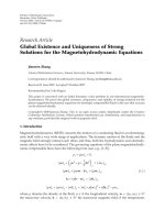
123


H. V. Long et al.

Fig. 1 Numerical simulation for fuzzy solution of (25)–(27) with Triangular fuzzy number [C]α = [0.1α +
0.9; 1.1 − 0.1α]

Example 5.2 The hyperbolic PDE is
u x y + u x + u y + u = f (x, y, c) = x y + cy + y + x + c + 1,

(28)

where (x, y) ∈ Ja × Jb = [0, 18 ] × [0, 18 ], c is a constant in J = [0, M], M > 0.
And the local condition are

u(0, 0) = u(x, 0) = 0; u(0, y) = cy.

(29)

We have a = b = 18 , p1 (x, y) = p2 (x, y) = c(x, y) = 1. We recognize that the right
side of the equation is f (x, y, c) = x y + cy + y + x + c + 1, so the hypothesis (H)
is satisfied with arbitrary positive number. So all conditions of the Theorem 4.1 hold.
Therefore there exists a unique fuzzy solution of this problem.
Indeed, for any fixed c ∈ [0, M], the deterministic solution of (28)–(29) is
u(x, y) = g(x, y, c) = cy + x y.
We fuzzify c, f and g by using the extension principle. Fuzzy function F is computed from f and G is computed from g. After that we will show that G is the fuzzy
solution of (24)–(25).
Indeed, let
[G]α = [g1 (x, y, α), g2 (x, y, α)] = [c1 (α)y + x y, c2 (α)y + x y]
and
[F]α = [ f 1 (x, y, α), f 2 (x, y, α)]
= [x y + c1 (α)y + y + x + c1 (α) + 1, x y + c2 (α)y + y + x + c2 (α) + 1] .
We consider differential operator
ϕ(Dx , D y )u(x, y) = u x y + u x + u y + u.

123


The existence and uniqueness of fuzzy solutions

Fig. 2 Numerical simulation for fuzzy solution of (28)–(29) with Gaussian fuzzy number [C]α =
[1 − 0.1 ln α1 , 1 + 0.1 ln α1 ]

We compute
[ϕ(Dx , D y )g1 (x, y, α), ϕ(Dx , D y )g2 (x, y, α)]

the result is
[x y + c1 (α)y + y + x + c1 (α) + 1, x y + c2 (α)y + y + x + c2 (α) + 1]
which are the α-cuts of fuzzy number x y + C y + y + x + C + 1. Hence G(x, y) is
differentiable and ϕ(Dx , D y )G(x, y, C) = F(x, y, C). Since all partials of G and F
with respect to c are positive and boundary conditions are all satisfied
g1 (0, 0, α) = g2 (0, 0, α) = 0, g1 (x, 0, α) = g2 (x, 0, α) = 0,
g1 (0, y, α) = c1 (α)y, g2 (0, y, α) = c2 (α)y.
Therefore, G(x, y, C) is the fuzzy solution of (28)–(29).
In this example, we fuzzify crisp number c by Gaussian fuzzy numbers C with
membership function C(t) = exp(−100(t − c)2 ). The α−cuts of C are
[c1 (α), c2 (α)] = c − 0.1 ln

1
1
, c + 0.1 ln
.
α
α

The continuity of extension principle states that fuzzy solution of (28)–(29) is
[G(x, y, C)]α =

c − 0.1 ln

1
α

y + x y, c + 0.1 ln

1

α

y + xy .

The simulation of some α-cuts of this fuzzy solution is shown in Fig. 2.

123