DSpace at VNU: A Minimized Assumption Generation Method for Component-Based Software Verification
Bạn đang xem bản rút gọn của tài liệu. Xem và tải ngay bản đầy đủ của tài liệu tại đây (320.37 KB, 10 trang )
IEICE TRANS. INF. & SYST., VOL.E93–D, NO.8 AUGUST 2010
2172
PAPER
A Minimized Assumption Generation Method for
Component-Based Software Verification∗
Ngoc Hung PHAM†a) , Viet Ha NGUYEN†b) , Toshiaki AOKI††c) , Nonmembers,
and Takuya KATAYAMA††d) , Fellow
SUMMARY
An assume-guarantee verification method has been recognized as a promising approach to verify component-based software by
model checking. This method is not only fitted to component-based software but also has a potential to solve the state space explosion problem in
model checking. The method allows us to decompose a verification target
into components so that we can model check each of them separately. In
this method, assumptions are seen as the environments needed for the components to satisfy a property and for the rest of the system to be satisfied.
The number of states of the assumptions should be minimized because the
computational cost of model checking is influenced by that number. Thus,
we propose a method for generating minimal assumptions for the assumeguarantee verification of component-based software. The key idea of this
method is finding the minimal assumptions in the search spaces of the candidate assumptions. The minimal assumptions generated by the proposed
method can be used to recheck the whole system at much lower computational cost. We have implemented a tool for generating the minimal assumptions. Experimental results are also presented and discussed.
key words: model checking, assume-guarantee reasoning, modular verification, learning algorithm, minimal assumption
1.
Introduction
Component-based development is one of the most important technical initiatives in software engineering because it
is considered an open, effective and efficient approach to reducing development cost and time while increasing software
quality. Component-based software (CBS) technology also
supports rapid development of complex evolving software
applications by enhancing reuse and adaptability. CBS can
be evolved by evolving one or more software components.
To realize such an ideal CBS paradigm, one of the
key issues is to ensure that those separately specified and
implemented components do not conflict with each other
when composed - the component consistency issue. The
current well-known technologies such as CORBA (OMG),
COM/DCOM or .NET (Microsoft), Java and JavaBeans
Manuscript received December 17, 2009.
Manuscript revised April 15, 2010.
†
The authors are with the College of Technology, Vietnam National University, Hanoi (VNU), 144 Xuan Thuy, Cau Giay, Hanoi,
Vietnam.
††
The authors are with the School of Information Science, Japan
Advanced Institute of Science and Technology (JAIST), Nomi-shi,
923–1292 Japan.
∗
This paper is an extension of our paper [10] presented at ICTAC’09.
a) E-mail:
b) E-mail:
c) E-mail:
d) E-mail:
DOI: 10.1587/transinf.E93.D.2172
(Sun), etc. only support component plugging. However,
components often fail to co-operate, i.e., the plug-and-play
mechanism fails. Currently, the popular solution to deal
with this problem is the verification of CBS by model checking [6]. Model checking is a practical approach for improving software reliability. It provides exhaustive state space
coverage for systems being checked and is particularly effective in detecting difficult coordination errors which frequently result from component composition. Nonetheless, a
major problem of model checking is the state space explosion.
In order to deal with the problem, a powerful method
called assume-guarantee verification was proposed in [7],
[12], [16], [17] by decomposing a verification target for a
component-based system into parts related to the individual components. The key idea of this method is to generate
assumptions as environments needed for components to satisfy a property. These assumptions are then discharged by
the rest of the system. For example, consider a simple case
where a CBS is made up of two components M1 and M2 .
The method proposed in [7] verifies whether this system satisfies a property p without composing M1 with M2 . For this
goal, an assumption A(p) is generated by applying a learning
algorithm called L* [2], [18] such that A(p) is strong enough
for M1 to satisfy p but weak enough to be discharged by M2
(i.e., A(p) M1 p and true M2 A(p) which are called
assume-guarantee rules, both hold). From these rules, this
system satisfies p. In order to check these assume-guarantee
rules, the number of states of the assumption A(p) should be
minimized because the computational cost of model checking of these rules is influenced by that number. This means
that the cost of verification of CBS is reduced with a smaller
assumption. Moreover, when a component is evolved after adapting some refinements in the context of the software
evolution, the whole evolved CBS including many existing
components and the evolved component is required to be
rechecked [9], [11]. In this case, we also can reduce the cost
of rechecking the evolved CBS by reusing the smaller assumption. These observations imply that the size of the generated assumptions is of primary importance. However, the
method proposed in [7], [8] focuses only on generating the
assumptions which satisfy the assume-guarantee rules. The
number of states of the generated assumptions is not mentioned in this work. Thus, the assumptions generated by the
method are not minimal. A more detailed discussion of this
issue can be found in Sect. 4.
Copyright c 2010 The Institute of Electronics, Information and Communication Engineers
PHAM et al.: A MINIMIZED ASSUMPTION GENERATION METHOD FOR COMPONENT-BASED SOFTWARE VERIFICATION
2173
This paper proposes a method for generating the
minimal assumptions for assume-guarantee verification of
component-based software to deal with the above issue. The
key idea of this method is finding the minimal assumption
that satisfies the assume-guarantee rules thus is considered
as a search problem in a search space of the candidate assumptions. These assumptions are seen as the environments
needed for components to satisfy a property and for the rest
of the CBS to be satisfied. With regard to the effectiveness,
the proposed method can generate the minimal assumptions
which have the minimal sizes and a smaller number of transitions than the assumptions generated by the method proposed in [7]. These minimal assumptions generated by the
proposed method can be used to recheck the whole CBS by
checking the assume-guarantee rules at much lower computational costs.
The paper is organized as follows. We first review
some background in Sect. 2. Section 3 describes the current
method for assumption generation by using the L* learning algorithm. Section 4 is about a minimized L*-based
assumption generation method to find the minimal assumptions for component-based software verification. Section 5
shows an implementation, experimental results, and discussion. Section 6 presents related works. Finally, we conclude
the paper in Sect. 7.
2.
Background
This section presents some basic concepts which are used in
our work as follows.
LTSs. This paper uses Labeled Transition Systems (LTSs)
to model behaviors of components. Let Act be the universal set of observable actions and let τ denote a local action
unobservable to a component’s environment. We use π to
denote a special error state. An LTS is defined as follows.
Definition 1: (LTS). An LTS M is a quadruple Q, αM, δ,
q0 where:
• Q is a non-empty set of states,
• αM ⊆ Act is a finite set of observable actions called
the alphabet of M,
• δ ⊆ Q × αM ∪ {τ} × Q is a transition relation, and
• q0 ∈ Q is the initial state.
Definition 2: (LTS Size).
Size of an LTS M =
Q, αM, δ, q0 is the number of states of M, denoted |M| (i.e.,
|M| = |Q|).
Definition 3: (Deterministic and Non-deterministic LTSs).
An LTS M = Q, αM, δ, q0 is non-deterministic if it contains τ-transition or if ∃(q, a, q′ ), (q, a, q′′ ) ∈ δ such that
q′ q′′ . Otherwise, M is deterministic.
Note 1: Let M = Q, αM, δ, q0 and M ′ = Q′ , αM ′ , δ′ , q′0 .
We say that M transits into M ′ with action a, denoted
M −→a M ′ if and only if (q0 , a, q′0 ) ∈ δ and αM = αM ′
and δ = δ′ . We use to denote the LTS {π}, Act, φ, π .
Traces. A trace σ of an LTS M is a sequence of observable
actions that M can perform starting at its initial state.
Definition 4: (Trace).
A trace σ of an LTS M =
Q, αM, δ, q0 is a finite sequence of actions a1 a2 . . . an , such
that there exists a sequence q0 q1 . . . qn , where for 1 ≤ i ≤ n,
(qi−1 , ai , qi ) ∈ δ.
Note 2: For Σ ⊆ Act, we use σ↑Σ to denote the trace obtained by removing from σ all occurrences of actions a
Σ. The set of all traces of M is called the language of M,
denoted L(M). Let σ = a1 a2 . . . an be a finite trace of an LTS
M. We use [σ] to denote the LTS Mσ = Q, αM, δ, q0 with
Q = {q0 , q1 , . . . , qn }, and δ = {(qi−1 , ai , qi )}, where 1 ≤ i ≤ n.
We say that an action a ∈ αM is enabled from a state s ∈ Q,
if there exists s′ ∈ Q, such that (s, a, s′ ) ∈ δ. Similarly, a
trace a1 a2 . . . an is enabled from s if there is a sequence of
states s0 , s1 , . . . , sn with s0 = s such that for 1 ≤ i ≤ n,
(si−1 , ai , si ) ∈ δ.
Parallel Composition. The parallel composition operator
is a commutative and associative operator that combines
the behavior of two models by synchronizing the actions
common to their alphabets and interleaving the remaining
actions.
Definition 5: (Parallel composition operator). The parallel composition between M1 = Q1 , αM1 , δ1 , q10 and M2 =
Q2 , αM2 , δ2 , q20 , denoted M1 M2 , is defined as follows. If
or M2 =
, then M1 M2 =
. Otherwise,
M1 =
M1 M2 is an LTS M = Q, αM, δ, q0 where Q = Q1 ×Q2 ,
αM = αM1 ∪ αM2 , q0 = (q10 , q20 ), and the transition relation
δ is given by the following rules:
(i)
α ∈ αM1 ∩ αM2 , (p, α, p′ ) ∈ δ1 , (q, α, q′ ) ∈ δ2
((p, q), α, (p′ , q′ )) ∈ δ
(1)
α ∈ αM1 \αM2 , (p, α, p′ ) ∈ δ1
((p, q), α, (p′ , q)) ∈ δ
(2)
α ∈ αM2 \αM1 , (q, α, q′ ) ∈ δ2
((p, q), α, (p, q′ )) ∈ δ
(3)
(ii)
(iii)
Example 1: When composing the two models represented
by two LTSs Input and Output illustrated in Fig. 2, the actions send and ack are synchronized and the others are interleaved.
Safety LTS, Safety Property, Satisfiability and Error
LTSs.
Definition 6: (Safety LTS). A safety LTS is a deterministic
LTS that contains no π states.
Definition 7: (Safety property.) A safety property asserts
that nothing bad happens. The safety property p is specified as a safety LTS p = Q, αp, δ, q0 whose language L(p)
defines the set of acceptable behaviors over αp.
Definition 8: (Satisfiability). An LTS M satisfies p, denoted as M |= p, if and only if ∀σ ∈ L(M): (σ↑αp) ∈ L(p).
IEICE TRANS. INF. & SYST., VOL.E93–D, NO.8 AUGUST 2010
2174
Note 3: When checking of the LTS M which satisfies the
property p, an error LTS, denoted perr , is created which traps
possible violations with the π state. perr is defined as follows:
Definition 9: (Error LTS). The error LTS of a property p =
Q, αp, δ, q0 is perr = Q ∪ {π}, αperr , δ′ , q0 , where αperr =
αp and δ′ = δ ∪ {(q, a, π) | a ∈ αp and ∄q′ ∈ Q : (q, a, q′ ) ∈
δ}.
Remark 1: The error LTS is complete, meaning each state
other than the error state has outgoing transitions for every
action in the alphabet. In order to verify a component M satisfying a property p, both M and p are represented by safety
LTSs, the parallel composition M perr is then computed. If
state π is reachable in the composition then M violates p.
Otherwise, it satisfies.
Deterministic Finite State Automata (DFAs). We use the
L* learning algorithm [2], [18] to generate a minimized assumption from two models and the required property. The
L* learning algorithm produces DFAs, which our work then
uses as LTSs.
Definition 10: (DFA). A DFA M is a five tuple Q, αM, δ,
q0 , F where:
• Q, αM, δ, q0 are defined as for deterministic LTSs, and
• F ⊆ Q is a set of accepting states.
Note 4: For a DFA M and a string σ, we use δ(q, σ) to
denote the state that M will be in after reading σ starting at
state q. A string σ is said to be accepted by a DFA M =
Q, αM, δ, q0 , F if δ(q0 , σ) ∈ F. The language of a DFA M
is defined as L(M) = {σ | δ(q0 , σ) ∈ F}.
Remark 2: A DFA M is prefix-closed if L(M) is prefixclosed (i.e., if v ∈ L(M), then any prefix of v is in L(M)).
The DFAs returned by the L* learning algorithm in the proposed method are unique, complete, minimal, and prefixclosed [18]. These DFAs therefore contain a single nonaccepting state. To get a safety LTS A from a DFA M, we
remove the non-accepting state denoted nas and all its ingoing transitions. Formally, for a DFA M= Q ∪ {nas}, αM, δ,
q0 , F , the safety LTS is chosen to be A = Q, αM, δ ∩ (Q ×
αM× Q), q0 .
Assume-Guarantee Reasoning. In the assume-guarantee
paradigm, a formula is a triple A(p) M p , where M is a
component, p is a property, and A(p) is an assumption about
M’s environment. The formula is true if whenever M is part
of a system satisfying A(p), then the system must also guarantee p. In our work, to check an assume-guarantee formula
A(p) M p , where both A(p) and p are safety LTSs, we
use a tool called LTSA [13] to compute A(p) M perr and
check if the error state π is reachable in the composition. If
it is, then the formula is violated, otherwise it is satisfied.
Definition 11: (Assumption). Given two models M1 and
M2 , and a required safety property p, A(p) is an assumption
if and only if it is strong enough for M1 to satisfy p but
Fig. 1
A framework for L*-based assumption generation.
weak enough to be discharged by M2 (i.e., A(p) M1 p
and true M2 A(p) , called assume-guarantee rules, both
hold). Equivalently, A(p) is an assumption if and only if
L(A(p) M1 )↑αp ⊆ L(p) and L(M2 )↑αA(p) ⊆ L(A(p)).
Remark 3: The iterative fashion for generating A(p) is illustrated in Fig. 1. Details of this fashion can be found in
[7]. An assumption with which the assume-guarantee rules
are guaranteed to return conclusive results is the weakest assumption AW defined in [8], which restricts the environment
of M1 no more and no less than necessary for p to be satisfied. The weakest assumption is defined as follows.
Definition 12: (Weakest assumption). Weakest assumption AW describes exactly those traces over the alphabet Σ =
(αM1 ∪αp)∩αM2 which, the error state π is not reachable in
the compositional system M1 perr . The weakest assumption
AW means that for any environment component E, M1 E|= p
if and only if E|=AW .
Minimal Assumption. The number of states of the assumptions generated by the current method for assume-guarantee
verification proposed in [7], [8], [12], [16] is not mentioned.
We define the concept of minimal assumption as follows.
Definition 13: (Minimal assumption). Given two models
M1 , M2 and a property p, A(p) is an assumption if and only
if A(p) satisfies the assume-guarantee rules. An assumption
A(p) represented by an LTS is minimal if and only if the
number of states of A(p) is less than or equal to the number
of states of any other assumptions.
3.
3.1
Assume-Guarantee Verification
The L* Learning Algorithm
The L* learning algorithms was developed by Angluin [2]
and later was improved by Rivest and Schapire [18]. L*
learns an unknown regular language and produces a DFA
that accepts it. The main idea of the L* learning algorithms is based on the “Myhill-Nerode Theorem” [14] in
PHAM et al.: A MINIMIZED ASSUMPTION GENERATION METHOD FOR COMPONENT-BASED SOFTWARE VERIFICATION
2175
the theory of formal languages. It said that for every regular set U⊆ Σ∗ , there exists a unique minimal deterministic
automata whose states are isomorphic to the set of equivalence classes of the following relation: w ≈w′ iff ∀u ∈ Σ∗ :
wu ∈ U ⇐⇒ w′ u ∈ U. Therefore, the main idea of L* is to
learn the equivalence classes, i.e., two prefix are not in the
same class if and only if there is a distinguishing suffix u.
Let U be an unknown regular language over some alphabet Σ. L* will produce a DFA M such that M is a
minimal deterministic automata corresponding to U and
L(M) = U. In order to learn U, L* needs to interact with a
Minimally Adequate Teacher, called Teacher. The Teacher
must be able to correctly answer two types of questions from
L*. The first type is a membership query, consisting of a
string σ ∈ Σ∗ ; the answer is true if σ ∈ U, and f alse otherwise. The second type of these questions is a conjecture,
i.e., a candidate DFA M whose language the algorithm believes to be identical to U. The answer is true if L(M) = U.
Otherwise the Teacher returns a counterexample, which is a
string σ in the symmetric difference of L(M) and U.
At a higher level, L* maintains a table T that records
whether string s in Σ∗ belong to U. It does this by making
membership queries to the Teacher to update the table. At
various stages L* decides to make a conjecture. It uses the
table T to build a candidate DFA Mi and asks the Teacher
whether the conjecture is correct. If the Teacher replies true,
the algorithm terminates. Otherwise, L* uses the counterexample returned by the Teacher to maintain the table with
string s that witness differences between L(Mi ) and U.
3.2 L*-Based Assumption Generation Method
The assume-guarantee paradigm is a powerful “divide-andconquer” mechanism for decomposing a verification process of a CBS into subtasks about the individual components. Consider a simple case where a system is made up of
two components including a framework M1 and an extension M2 . The goal is to verify whether this system satisfies
a property p without composing M1 with M2 . For this purpose, an assumption A(p) is generated [7] by applying the
L* learning algorithm such that A(p) is strong enough for
M1 to satisfy p but weak enough to be discharged by M2
(i.e., A(p) M1 p and true M2 A(p) both hold). From
these assume-guarantee rules, this system satisfies p.
In order to obtain appropriate assumptions, this method
applies the assume-guarantee rules in an iterative fashion illustrated in Fig. 1. At each iteration i, a candidate assumption Ai is produced based on some knowledge about the
system and the results of the previous iteration. The two
steps of the assume-guarantee rules are then applied. Step 1
checks whether M1 satisfies p in an environment that guarantees Ai by computing formula Ai M1 p . If the result is
f alse, it means that this candidate assumption is too weak.
The candidate assumption Ai therefore must be strengthened
with the help of the counterexample cex produced by this
step. Otherwise, the result is true, it means that Ai is strong
enough for the property to be satisfied. The step 2 is then
applied to check that if component M2 satisfies Ai by computing formula true M2 Ai . If this step returns true, the
property p holds in the compositional system M1 M2 and
the algorithm terminates. Otherwise, this step returns f alse;
further analysis is required to identify whether p is indeed
violated in M1 M2 or the candidate Ai is too strong to be
satisfied by M2 . Such analysis is based on the counterexample cex returned by this step. The L* algorithm must
check that the counterexample cex belong to the unknown
language U = L(AW ). If it does not, the property p does not
hold in the system M1 M2 . Otherwise, Ai is too strong. The
candidate assumption Ai must be weakened (i.e., behaviors
must be added with the help of cex) in iteration i + 1. A
new candidate assumption may of course be too weak, and
therefore the entire process must be repeated.
4.
Minimized Assumption Generation Method
As mentioned in Sect. 1, the assumptions generated by the
method proposed in [7] are not minimal. Figure 2 is a counterexample to prove this fact. In this counterexample, given
two component models M1 (Input) and M2 (Output), and a
required property p, the method proposed in [7] generates
the assumption A(p). In order to learn the language of A(p),
the method uses L* to learns the language of the weakest
assumption AW over the alphabet Σ = (αM1 ∪ αp) ∩ αM2
and produces a DFA that accepts it. For this purpose, L*
builds an observation table (S , E, T ) where S and E are a
set of prefixes and suffixes respectively, both over Σ∗ . T is
a function which maps (S ∪ S .Σ).E to {true, f alse}, where
the operator “.” is defined as follows.
Definition 14: (Operation “.”). Given two sets of event sequences P and Q, P.Q = {pq | p ∈ P, q ∈ Q}, where pq
presents the concatenation of the event sequences p and q.
The function for answering membership queries used
in the method proposed in [7] is defined as follows.
Definition 15: (Function for answering membership queries).
Given an observation table (S , E, T ), T is a function which
maps (S ∪ S .Σ).E to {true, f alse} such that for any string s ∈
(S ∪ S .Σ).E, T (s) = true if s ∈ L(AW ), and f alse otherwise.
Fig. 2 A counterexample proves that the assumptions generated in [7]
are not minimal.
IEICE TRANS. INF. & SYST., VOL.E93–D, NO.8 AUGUST 2010
2176
function which maps (S ∪ S .Σ).E to {true, f alse, “?”} such
that for any string s ∈ (S ∪ S .Σ).E, if s is the empty string
(s = λ) then T (s) = true, else T (s) = f alse if s L(AW ),
and “?” otherwise.
Fig. 3 The reason shows why the assumptions generated in [7] are not
minimal.
However, there is a smaller assumption with a smaller
size and a smaller number of transitions shown in Fig. 2.
The reason why this method does not generate a minimal assumption is presented in Fig. 3. In this figure, if s ∈ L(AW )
but s L(Am (p)) (the minimized assumption), then T (s) is
set to true (in this case, T (s) should be f alse). For this reason, the assumption A(p) generated by this method contains
such strings/traces which do not belong to the language of
the minimized assumption being learned.
This section proposes a method for generating minimal assumptions for assume-guarantee verification of
component-based software. We also define a new technique
for answering membership queries to deal with the above issue. The minimal assumption is generated by combining the
L* learning algorithm and the breadth-first search strategy.
We prove that the assumptions generated by this method are
minimal (Theorem 2).
4.1 An Improved Technique for Answering Membership
Queries
As mentioned above, in order to learn the language of the
assumption, the L* learning algorithm used in [7] builds
an observation table (S , E, T ) where T is a function which
maps (S ∪ S .Σ).E to {true, f alse}. For any string s ∈ (S ∪
S .Σ).E, T (s) = true if s ∈ L(AW ), and f alse otherwise. In
the case where s ∈ L(AW ), we cannot ensure that whether s
belongs to the language being learned or not (i.e., whether
s ∈ L(A(p))?). If s L(A(p)) then T (s) should be f alse.
However, the work in [7] set T (s) to true in this case. For
this reason, the generated assumptions are not minimal in
this work. In order to solve this issue, we use a new value
called “?” to represent the value of T (s) in such cases. We
define an improved technique for answering membership
queries as follows. To generate a minimal assumption, the
L* learning algorithm used in our work builds an observation table (S , E, T ), where S and E are a set of prefixes and
suffixes respectively, both over Σ∗ . T is a function which
maps (S ∪ S .Σ).E to {true, f alse, “?”}, where “?” can be
seen as “don’t know” value. The “don’t know” value means
that for each string s ∈ (S ∪ S .Σ).E, even if s ∈ L(AW ),
we do not know whether s belongs to the language of the
assumption being learned or not. The function for answering membership queries used in our method is defined as
follows.
Definition 16: (Improved function for answering membership queries). Given an observation table (S , E, T ), T is a
4.2
Minimal Assumption Generation
Finding an assumption where it has a minimal size that satisfies the assume-guarantee rules thus is considered as a
search problem in a search space of observation tables. We
use the breadth-first search strategy because this strategy ensures that the generated assumption is minimal (Theorem 2).
The following is more detailed presentation of the
proposed algorithm for generating the minimal assumption
shown in Algorithm 1. In this algorithm, we use a queue
data structure which contains the generated observation tables with the first-in first-out order. These observation tables
are used for generating the candidate assumptions. Initially,
the algorithm sets the queue q to the empty queue (line 1).
We then put the initial observation table OT 0 = (S 0 , E0 , T 0 )
into the queue q as the root of the search space of observation tables, where S 0 = E0 = {λ} (λ represents the empty
string) (line 2). Subsequently, the algorithm gets a table OT i
from the top of the queue q (line 4). If OT i contains the
“don’t know” value “?” (line 5), we obtain all instances of
OT i by replacing all “?” entries in OT i with both true and
f alse (line 6). For example, the initial observation table of
the illustrative system presented in Fig. 2 and one of its instance obtained by replacing all “?” entries with true value
are showed in Fig. 4. The obtained instances then are put
into the queue q (line 7). Otherwise, the table OT i does not
contain the “?” value (line 9). In this case, if OT i is not
closed (line 10), an updated table OT is obtained by calling the procedure named make closed(OT i ) (line 11). OT
then is put into q (line 12). In the case where the table OT i
is closed (line 13), a candidate assumption Ai is generated
from OT i (line 14). The candidate assumption Ai is used
to check whether it satisfies the two steps of the assumeguarantee rules. The step 1 is applied by calling the procedure named S tep1(Ai ) to check whether M1 satisfies p in an
environment that guarantees Ai by computing the formula
Ai M1 p . If S tep1(Ai ) fails with a counterexample cex
(line 15), Ai is too weak for M1 to satisfy p. Thus, the candidate assumption Ai must be strengthened by adding a suffix
e of cex that witnesses a difference between L(Ai ) and the
language of the assumption being learned to Ei of the table
OT i (line 16). After that, an updated table OT is obtained
by calling the procedure named update(OT i ) (line 17). OT
then is put into q (line 18). Otherwise, S tep1(Ai ) return true
(line 19). This means that Ai is strong enough for M1 to
satisfy the property p. The step 2 is then applied by calling
the procedure named S tep2(Ai ) to check that if M2 satisfies
Ai by computing the formula true M2 Ai . If S tep2(Ai )
fails with a counterexample cex (line 20), further analysis is
required to identify whether p is indeed violated in M1 M2
or Ai is too strong to be satisfied by M2 . Such analysis is
PHAM et al.: A MINIMIZED ASSUMPTION GENERATION METHOD FOR COMPONENT-BASED SOFTWARE VERIFICATION
2177
Algorithm 1 Minimized assumption generation.
Input: M1 , M2 , p: two models M1 and M2 , and a required property p
Output: Am (p) or cex: an assumption Am (p) with a smallest size if M1 M2
satisfies p, and a counterexample cex otherwise
1: Initially, q = empty {q is an empty queue}
2: q.put(OT 0 ) {OT 0 = (S 0 , E0 , T 0 ), S 0 = E0 = {λ}, where λ is the empty
string}
3: while q empty do
4:
OT i = q.get() {getting OT i from the top of q}
5:
if OT i contains “?” value then
6:
for each instance OT of OT i do
7:
q.put(OT ) {putting OT into q}
8:
end for
9:
else
10:
if OT i is not closed then
11:
OT = make closed(OT i )
12:
q.put(OT )
13:
else
14:
construct a candidate DFA Ai from the closed OT i
15:
if S tep1(Ai ) fails with cex then
16:
add the suffix e of the counterexample cex to Ei
17:
OT = update(OT i )
18:
q.put(OT )
19:
else
20:
if S tep2(Ai ) fails with cex then
21:
if cex witnesses violation of p then
22:
return cex
23:
else
24:
add the suffix e of the counterexample cex to Ei
25:
OT = update(OT i )
26:
q.put(OT )
27:
end if
28:
else
29:
return Ai
30:
end if
31:
end if
32:
end if
33:
end if
34: end while
based on the counterexample cex. If cex witnesses the violation of p in the system M1 M2 (line 21), the algorithm
terminates and returns cex (line 22). Otherwise, Ai is too
strong to be satisfied by M2 (line 23). The candidate assumption Ai therefore must be weakened by adding a suffix
e of cex to Ei of the table OT i (line 24). After that, an updated table OT is obtained by calling the procedure named
update(OT i ) (line 25). OT then is put into q (line 26). Otherwise, S tep2(Ai ) return true (line 28). This means that the
property p holds in the compositional system M1 M2 . The
algorithm terminates and returns Ai as the minimal assumption (line 29). The algorithm iterates the entire process by
looping from line 3 to line 34 until the queue q is empty or
a minimal assumption is generated.
Example 2: Given M1 , M2 , and the required property p
shown in Fig. 2, the Algorithm 1 starts to generate a minimal assumption from the initial observation table presented
in Fig. 4. At the first iteration, the algorithm produces A1
shown in Fig. 5 as a candidate minimal assumption. The
step 1 is applied and the procedure S tep1(A1 ) fails with a
Fig. 4
The initial observation table and one of its instances.
Fig. 5
The generated candidate assumptions.
counterexample cex = send ack. A suffix e = ack is added
to E1 for producing the next candidate assumption A2 presented in Fig. 2. This candidate satisfies both steps in the
algorithm (S tep1(A2 ) and S tep2(A2 ) return true). Therefore, the proposed algorithm terminates and returns A2 as
the minimal assumption.
Characteristics of the Search Space. The search space of
observation tables used in the proposed method exactly contains the generated observation tables which are used to generate the candidate assumptions. This search space is seen
as a search tree where its root is the initial observation table
OT 0 . We can conveniently define the size of an observation table OT = (S, E, T) as |S|, denoted |OT |. We use Ai j to
denote the jth candidate assumption generated from the jth
observation table (denoted OT i j ) at the depth i of the search
tree. From the way to build the search tree presented in Algorithm 1 we have a theorem as follows.
Theorem 1: Let Ai j and Akl be two candidate assumptions
generated at the depth i and k respectively. |Ai j | < |Akl | implies that i < k.
Proof. The observation tables at the depth i+1 are generated
from the observation tables at the depth i exactly in one of
the following cases:
• There is at least a table OT i j of the tables at the depth i
which contains the “?” value. In this case, the instances
of this table are the tables at the depth i+1. These tables
have the same size with the table OT i j .
• There is at least a table OT i j of the tables at the depth
i which is not closed. An updated table OT (i+1)k at the
depth i+1 is obtained from this table by adding a new
element to S i j . This mean that |OT i j | < |OT (i+1)k |.
• Finally, there is at least a table OT i j of the tables at
the depth i which is not an actual assumption. In this
case, an updated table OT (i+1)k at the depth i+1 is obtained from this table by adding a suffix e of the given
counterexample cex to Ei j . This mean that |OT i j | =
|OT (i+1)k |.
These observations imply that if the size of the candi-
IEICE TRANS. INF. & SYST., VOL.E93–D, NO.8 AUGUST 2010
2178
date generated from a table at the depth i less than the size
of the candidate generated from a table at the depth k, then
i < k.
these tools for some illustrative systems. We also discuss
the advantages and disadvantages of the proposed method.
5.1
4.3 Termination and Correctness
Termination and correctness of the proposed algorithm
for the minimized assumption generation showed in Algorithm 1 are proved by the following theorem.
Theorem 2: Given two component models M1 and M2 ,
and a property p, the proposed algorithm for the minimized
assumption generation presented in Algorithm 1 terminates
and returns true and an assumption Am (p) with a minimal
size such that it is strong enough for M1 to satisfy p but
weak enough to be discharged by M2 , if the compositional
system M1 M2 satisfies p, and f alse otherwise.
Proof. At any iteration, the proposed method returns true
or f alse (i.e., the compositional system M1 M2 violates p)
and terminates or continues by providing a counterexample
or continues to update the current observation table (if this
table contains “?” or it is not closed). Because the proposed
method is based on the L* learning algorithm, by the correctness of L* [2], [18], we ensure that if the L* learning algorithm keeps receiving counterexamples, in the worst case,
the algorithm will eventually produce the weakest assumption AW and terminates, by the definition of AW [8]. This
means that the search space exactly contains the observation table OT W which is used to generate AW . In the worst
case, the proposed method reaches to OT W and terminates.
With regard to correctness, the proposed method uses
two steps of the assume-guarantee rules (i.e., Ai M1 p
and true M2 Ai ) to answer the question of whether the
candidate assumption Ai produced by the method is an actual assumption or not. It only returns true and a minimal assumption Am (p) = Ai when both steps return true,
and therefore its correctness is guaranteed by the assumeguarantee rules. The proposed method returns a real error
when it detects a trace σ of M2 which violates the property p when simulated on M1 . In this case, it implies that
M1 M2′ violates p. The remaining problem is to prove that
the assumption Am (p) generated by the proposed method is
minimal. Suppose that there exists an assumption A such
that |A| < |Am (p)|. By using Theorem 1 for this fact, we can
imply that the depth of the table used to generate A less than
the depth of the table used to generate Am (p). This means
that the table used to generate A has been visited by our algorithm. In this case, the algorithm has generated A as a
candidate assumption and A was not an actual assumption.
These facts imply that such assumption A does not exist.
5.
Experiment and Discussion
This section presents our implemented tools for L*-based
assumption generation and experimental results by applying
Experiment
In order to evaluate the effectiveness of the proposed
method, we have implemented the assumption generation
method proposed in [7] and the proposed minimized assumption generation method in the Objective Caml (OCaml)
functional progamming language [15]. We tested our
method by using several illustrative systems and compared
the method with that proposed in [7]. The applied systems are the typical concurrent system Input/Output channel
(I/O ver.1) and its evolved versions (I/O ver.2 and I/O ver.3)
shown in [9], gas oven control system (GOCS), and banking
subsystem (BS).
The size (Ass. Size), the number of transitions
(Trans. of Ass.), and the generating time of the generated
assumptions are evaluated in this experiment. We also evaluate the rechecking time for each system by reusing the
generated assumptions for checking the assume-guarantee
rules. Table 1 shows experimental results for this purpose.
In the results, the system size (Sys. Size) is the product of
the sizes of the software components and the size of the required property for each CBS. Our obtained experimental
results imply that the generated minimal assumptions have
smaller sizes and number of transitions than the generated
ones by the method proposed in [7]. These minimal assumptions are effective for rechecking the systems with a lower
cost. However, our method has a higher cost for generating
the assumption.
We also use the tool for verifying concurrent systems called LTSA [13] to check correctness of the minimal assumption Am (p) which is generated by our proposed
method. For this purpose, we check that whether Am (p) satisfies the assume-guarantee rules (i.e., Am (p) M1 p and
true M2 Am (p) both hold) by checking the compositional
systems Am (p) M1 perr and M2 Am (p)err in the LTSA tool.
For each compositional system, the LTSA tool returns the
same result as our verification result for each system.
The implemented tool and the illustrative systems
which are used in our experimental results is available at
the site [1].
5.2
Discussion
With regard to the importance of the minimal assumptions,
obtaining smaller assumptions is interesting for several advantages as follows:
• Modular verification of CBS is done by model checking the assume-guarantee rules which has the assumption as one of its components. The computational cost
of this checking is influenced by the size of the assumption. This means that the cost of verification of CBS is
reduced with a smaller assumption which has a smaller
size and smaller number of transitions.
PHAM et al.: A MINIMIZED ASSUMPTION GENERATION METHOD FOR COMPONENT-BASED SOFTWARE VERIFICATION
2179
Table 1
System
I/O ver. 1
I/O Ver. 2
I/O Ver. 3
GOCS
BS
Sys.
Size
18
18
75
180
1200
Ass.
Size
2
4
3
14
13
Experimental results.
The Current AG Method
Trans.
Generating
Rechecking
of Ass.
Time (ms)
Time (ms)
4
93
7.8
9
97
9.5
12
94
37.5
110
118
34.5
102
94
33
• When a component is evolved after adapting some refinements in the context of the software evolution, the
whole evolved CBS of many existing components and
the evolved component is required to be rechecked [9],
[11]. In this case, we can reduce the cost of rechecking
the evolved CBS by reusing the smaller assumption.
• Finally, a smaller assumption means less complex behavior so this assumption is easier for a human to understand. This is interesting for checking the largescale systems.
The experimental results show that the difference between the generating time in our method and the current
method is not so much because the systems used in our experiment are small. In fact, the method proposed in [7] always generates the assumptions at a lower generating time.
If we are not interesting in the above advantages, the method
proposed in [7] is better than our method for generating assumptions. Otherwise, the generated assumptions are used
for rechecking the CBS or are reused for regenerating the
new assumptions for rechecking the evolved CBS [9], [11].
In this case, the minimal assumptions generated by our
method are useful. However, the breadth-first-search which
is used in our work, may be not practical because it consumed too much memory. For larger systems, the computational cost for generating the minimal assumption is very
expensive. An idea to solve this issue is using the iterativedeepening depth first search. The search strategy combines
the space efficiency of the depth-first search with the optimality of breadth-first search. It proceeds by running a
depth-limited depth-first search repeatedly, each time increasing the depth limit by one. The assumptions generated
by using this search strategy are smaller than the assumption generated in [7] but they may be not minimal. Another
problem in the proposed method is that the queue has to hold
an exponentially growing of the number of the observation
tables. This makes our method unpractical for large-scale
systems. In order to reduce the search space of the observation tables, we improve the technique for answering membership queries to reduce the number of instances of each
table which contains the “?” entries. At any step i of the
learning process, if the current candidate assumption Ai is
too strong for M2 to be satisfied, then L(Ai ) is exactly a subset of the language of the assumption being learned. For
every s ∈ (S ∪ S.Σ).E, if s ∈ L(AW ) and s ∈ L(Ai ), instead
of setting T(s) to “?”, we should set T(s) to true. We can
reduce several number of the “?” entries by reusing such
candidate assumptions.
Ass.
Size
2
2
3
6
12
Minimized AG Method
Trans.
Generating
Rechecking
of Ass.
Time (ms)
Time (ms)
3
94
7.6
4
102
6.3
6
107
23.5
26
120
24.8
48
109
23.5
Moreover, the proposed method focuses on minimizing the size of the generated assumption. The generated
minimal assumption does not correspond to the strongest
assumption which satisfies the assume-guarantee rules. Instead of focusing on the size, it should be better to focus on
the weakness of the generated assumption.
Finally, though the proposed method considers the simple case where the CBS only consists of two components M1
and M2 , we can generalize it for a larger CBS containing ncomponents M1 , M2 , . . . , Mn (n ≥ 2). In order to apply the
method for the such CBS, we can consider the CBS as a
software system which contains two components, i.e., the
compositional component M1 M2 . . . Mn−1 and Mn . The
method for larger CBS consists of the similarly steps as described in Algorithm 1.
6.
Related Work
There are many works that have been recently proposed in
assume-guarantee verification of component-based systems,
by several authors. Focusing only on the most recent and
closest ones we can refer to [3], [7], [8], to [5], and [4], [9],
[11].
D. Giannakopoulou et al. proposes an algorithm for automatically generating the weakest possible assumption for
a component to satisfy a required property [8]. Although the
motivation of this work is different, the ability to generate
the weakest assumption can be used for assume-guarantee
verification of component-based software. Based on this
work, the work proposed in [7] presents a framework to
generate a stronger assumption incrementally and may terminate before the weakest assumption is computed. The key
idea of the framework is to generate assumptions as environment for components to satisfy the property. The assumptions are then discharged by the rest of the CBS. However,
this framework focuses only on generating the assumptions.
The number of states of the generated assumptions is not
mentioned in this work. Thus, the assumptions generated
by this work are not minimal. This work has been extended
in [3] for modular verification of component-based systems
at the source code level. Our work improves these works
to generate the minimal assumptions in order to reduce the
computational cost for rechecking the CBS.
An approach about optimized L*-based assumeguarantee reasoning was proposed by Chaki et al. [5]. The
work suggests three optimizations to the L*-based automated assume-guarantee reasoning algorithm for the com-
IEICE TRANS. INF. & SYST., VOL.E93–D, NO.8 AUGUST 2010
2180
positional verification of concurrent systems. The purposes
of this work is to reduce the number of the membership
queries and the number of the candidate assumptions which
are used for generating the assumption, and to minimize the
alphabet used by the assumption. However, the core of this
approach is the framework proposed in [7]. Thus, the assumptions generated by this work are not minimal. Our
work and this work share the motivation for optimizing the
framework presented in [7] but we focus on generating the
minimal assumptions.
Finally, several works for assume-guarantee verification of evolving software were suggested in [4] and our previous works [9], [11]. The work in [4] focuses on component substitutability directly from the verification point of
view. The purpose of this work is to provide an effective verification procedure that decides whether a component can
be replaced with a new one without violation. The work
improves the L* algorithm to an improved version called
the dynamic L* algorithm by reusing the previous assumptions. However, this work assumes the availability and correctness of models that describe the behaviors of the software components. Our previous works proposed in [9],
[11] were suggested to deal with this issue by providing a
method for updating the inaccurate models of the evolved
component. These updated models then are used to verify
the evolved CBS by applying the improved L* algorithm.
Even these works improve the L* algorithm to optimize it,
the core of these works is the framework proposed in [7].
As a result, the assumptions generated by these works are
not minimal. On the contrary, we focus on generating the
minimal assumptions. The minimal assumptions generated
by our work may be useful for these works to recheck the
evolved at much lower computational costs.
7.
Conclusion
We have presented a method for generating minimal assumptions for assume-guarantee verification of componentbased software. The key idea of this method is finding the
minimal assumptions in the search space of the candidate
assumptions. These assumptions are strong enough for the
components to satisfy a property and weak enough to be
satisfied by the rest of the component-based software. In
this method, we have improved the technique for answering
membership queries of the Teacher which helps the L* to
correctly answer the membership query questions by using
the “don’t know” value. By using this technique, the proposed method ensures that every trace which belongs to the
language of the generated assumption precisely corresponds
to a trace in the language being learned. The search space
of observation tables used in the proposed method exactly
contains the generated observation tables which are used to
generate the candidate assumptions. This search space is
seen as a search tree where its root is the initial observation
table. Finding an assumption with a minimal size such that
it satisfies the assume-guarantee rules thus is considered a
search problem in this search tree. We apply the breadth-
first search strategy because this strategy ensures that the
generated assumptions are minimal (see Theorem 2). The
minimal assumptions generated by the proposed method can
be used to recheck the whole component-based software at
a lower computational cost. We have also implemented a
tool for the assumption generation method proposed in [7]
and our minimized assumption generation method. This implementation is used to verify some illustrative componentbased software to show the effectiveness of the proposed
method.
We are investigating how to generalize the proposed
method for larger CBS, i.e., CBS containing more than two
components. We are also improving our method and applying some CBS with their sizes are larger than the sizes of the
CBS which are used in our experiment to show the practical
usefulness of our proposed method. Moreover, although our
work focuses only on checking the safety properties of CBS,
we are going to extend the proposed method for checking
other properties, e.g., liveness properties and apply the proposed method for general systems, e.g., hardware systems.
Acknowledgments
This work is partly supported by the research project
No. QGTD 09.02 granted by Vietnam National University,
Hanoi.
References
[1] A minimized assumption generation tool for modular verification of
component-based software,
s0620204/MAGTool/, 2009.
[2] D. Angluin, “Learning regular sets from queries and counterexamples,” Inf. Comput., vol.75, no.2, pp.87–106, Nov. 1987.
[3] C. Blundell, D. Giannakopoulou, and C. Pasareanu, “Assumeguarantee testing,” Proc. 4th Microsoft Research – Specification and
Verification of Component-Based Systems Workshop (SAVCBS),
pp.7–14, Portugal, Sept. 2005.
[4] S. Chaki, N. Sharygina, and N. Sinha, “Verification of evolving software,” Proc. 3rd Microsoft Research – Specification and Verification of Component-Based Systems Workshop, pp.55–61, California,
USA, Nov. 2004.
[5] S. Chaki and O. Strichman, “Three optimizations for assumeguarantee reasoning with L*,” Formal Methods in System Design,
vol.32, no.3, pp.267–284, June 2008.
[6] E.M. Clarke, O. Grumberg, and D. Peled, Model Checking, The
MIT Press, 1999.
[7] J.M. Cobleigh, D. Giannakopoulou, and C. Pasareanu, “Learning assumptions for compositional verification,” Proc. 9th TACAS,
pp.331–346, Poland, April 2003.
[8] D. Giannakopoulou, C. Pasareanu, and H. Barringer, “Assumption
generation for software component verification,” Proc. 17th IEEE
Int. Conf. on Automated Softw. Eng., pp.3–12, Edinburgh, UK,
Sept. 2002.
[9] P.N. Hung, T. Aoki, and T. Katayama, “Modular conformance
testing and assume-guarantee verification for evolving componentbased software,” IEICE Trans. Fundamentals, vol.E92-A, no.11,
pp.2772–2780, Nov. 2009.
[10] P.N. Hung, T. Aoki, and T. Katayama, “A minimized assumption generation method for component-based software verification,”
Proc. 6th International Colloquium on Theoretical Aspects of Computing (ICTAC), LNCS 5684, pp.277–291, Springer-Verlag Berlin
PHAM et al.: A MINIMIZED ASSUMPTION GENERATION METHOD FOR COMPONENT-BASED SOFTWARE VERIFICATION
2181
Heidelberg, Aug. 2009.
[11] P.N. Hung and T. Katayama, “Modular conformance testing and
assume-guarantee verification for evolving component-based software,” Proc. 15th Asia-Pacific Softw. Eng. Conf. (APSEC), IEEE
Computer Society, pp.479–486, Washington, DC, Dec. 2008.
[12] C.B. Jones, “Tentative steps toward a development method for interfering programs,” ACM Trans. Programming Languages and Systems (TOPLAS), vol.5, no.4, pp.596–619, Oct. 1983.
[13] J. Magee and J. Kramer, Concurrency: State Models & Java Programs, John Wiley & Sons, 1999.
[14] A. Nerode: “Linear automaton transformations,” Proc. American
Mathematical Society, no.9, pp.541–544, 1958.
[15] French national institute for research in computer science and control (INRIA), Objective caml,
2004.
[16] A. Pnueli, “In transition from global to modular temporal reasoning about programs,” in Logics and Models of Concurrent Systems,
ed. K.R. Apt, Nato Asi Series F: Computer and Systems Sciences,
vol.13, pp.123–144, Springer-Verlag New York, 1985.
[17] E.W. Stark, “A proof technique for rely/guarantee properties,” Proc.
5th Conf. on Found. of Soft. Tech. and Theoretical Computer Science, pp.369–391, 1985.
[18] R.L. Rivest and R.E. Schapire, “Inference of finite automata using
homing sequences,” Inf. Comput., vol.103, no.2, pp.299–347, April
1993.
Ngoc Hung Pham
received his B.S. degree from College of Technology, Vietnam National University, Hanoi (2002), M.S. and PhD.
degrees from Japan Advanced Institute of Science and Technology (2006, 2009). He is now a
lecturer at College of Technology, Vietnam National University, Hanoi. His research interests
include model checking, assume-guarantee verification, conformance testing, and software evolution.
Viet Ha Nguyen
received his B.S., M.S.,
and PhD. degrees from Takushoku University
(1997, 1999, 2002). He is now a lecturer at College of Technology, Vietnam National University, Hanoi. His research interests include software architecture and software verification.
Toshiaki Aoki
is an associate professor,
JAIST(Japan Advanced Institute of Science and
Technology). He received B.S. degree from Science University of Tokyo(1994), M.S. and Ph.D.
degrees from (1996, 1999). He was an associate
at JAIST from 1999 to 2006, and a researcher of
PRESTO/JST from 2001-2005. His research interests include formal methods, formal verification, theorem proving, model checking, objectoriented design/analysis, and embedded software.
Takuya Katayama
received Ph.D degree
in Electrical Engineering from Tokyo Institute
of Technology in 1971. He has been a professor
there in the Department of Computer Science
until 1996. He was a professor in the school
of Information Science at Japan Advanced Institute of Science and Technology from1991 to
2007 and is now president. He has been working
on software process and its environment, software evolution and formal approach in software
engineering.