DSpace at VNU: Lattice quantum chromodynamics at the physical point and beyond

Prog. Theor. Exp. Phys. 2012, 01A102 (31 pages)
DOI: 10.1093/ptep/pts002

Lattice quantum chromodynamics at the physical
point and beyond
S. Aoki1,2 , N. Ishii1 , K.-I. Ishikawa3 , N. Ishizuka1,2 , T. Izubuchi4 , D. Kadoh5 , K. Kanaya1 ,
Y. Kuramashi1,2,6 , Y. Namekawa2 , O. H. Nguyen7 , M. Okawa3 , K. Sasaki8 , Y. Taniguchi1,2 ,
A. Ukawa2 , N. Ukita2 , T. Yamazaki9 , and T. Yoshié1,2 (PACS-CS Collaboration)
1

Faculty of Pure and Applied Sciences, University of Tsukuba, Tsukuba, Ibaraki 305-8571, Japan
Center for Computational Sciences, University of Tsukuba, Tsukuba, Ibaraki 305-8577, Japan
3
Graduate School of Science, Hiroshima University, Higashihiroshima, Hiroshima 739-8526, Japan
4
RIKEN BNL Research Center, Brookhaven National Laboratory, Upton, NY 11973, USA
5
RIKEN, Wako, Saitama 351-01, Japan
6
RIKEN Advanced Institute for Computational Science, Kobe 650-0047, Japan
7
Department of Physics, College of Natural Science, Vietnam National University, Hanoi, Vietnam
8
Graduate School of Science, Tokyo Institute of Technology, Meguro, Tokyo 152-8550, Japan
9
Kobayashi-Maskawa Institute for the Origin of Particles and the Universe, Nagoya University, Nagoya
464-8602, Japan
2

...............................................................................
We review the work of the PACS-CS Collaboration, which aimed to realize lattice quantum

chromodynamics (QCD) calculations at the physical point, i.e., those with quark masses set
at physical values. This has been a long-term goal of lattice QCD simulation since its inception
in 1979. After reviewing the algorithmic progress, which played a key role in this development,
we summarize the simulations that explored the quark mass dependence of hadron masses down
to values close to the physical point. In addition to allowing a reliable determination of the light
hadron mass spectrum, this work provided clues on the validity range of chiral perturbation theory, which is widely used in phenomenology. We then describe the application of the technique of
quark determinant reweighting, which enables lattice QCD calculations exactly on the physical
point. The physical quark masses and the strong coupling constants are fundamental constants
of the strong interaction. We describe a non-perturbative Schrödinger functional approach to
figure out the non-perturbative renormalization needed to calculate them. There are a number of
physical applications that can benefit from lattice QCD calculations carried out either near or at
the physical point. We take up three illustrative examples: calculation of the physical properties
of the ρ meson as a resonance, the electromagnetic form factor and charge radius of the pion,
and charmed meson spectroscopy. Bringing single hadron properties under control opens up a
number of new areas for serious lattice QCD research. One such area is electromagnetic effects
in hadronic properties. We discuss the combined QCD plus QED simulation strategy and present
results on electromagnetic mass difference. Another area is multi-hadron states, or nuclei. We
discuss the motivations and difficulties in this area, and describe our work for deuteron and
helium as our initial playground. We conclude with a brief discussion on the future perspective
of lattice QCD.
.................................................................................................

© The Author(s) 2012. Published by Oxford University Press on behalf of the Physical Society of Japan.
This is an Open Access article distributed under the terms of the Creative Commons Attribution License ( />which permits unrestricted use, distribution, and reproduction in any medium, provided the original work is properly cited.

Downloaded from at California Institute of Technology on July 3, 2015

Received April 29, 2012; Accepted May 28, 2012; Published August 29, 2012

PTEP 2012, 01A102

1.

S. Aoki et al.

Introduction

2/31

Downloaded from at California Institute of Technology on July 3, 2015

Lattice quantum chromodynamics (QCD) has close to four decades of history [1], and numerical simulation of lattice QCD has now been pursued for over 30 years [2–6]. Despite the promise that it would
provide a first-principles method for extracting physical predictions from the basic Lagrangian of
QCD, lattice QCD simulation in practice suffered from restrictions due to the need for various approximations and extrapolations. Efforts over the past three decades have removed these restrictions one
by one, and numerical lattice QCD has now reached the point where calculations are possible directly
at the physical point with light up, down, and strange quark masses taking physical values. We believe
that this is a turning point in lattice QCD research. The purpose of the present article is to review our
effort to achieve this goal, to present physics results obtained along the way [7–18], and to discuss
future directions.
In order to place our work in a historical perspective, let us discuss the situation of lattice QCD
simulation leading up to the middle of the 2000s when the work to be reviewed here was started.
There have been five sources of systematic errors which have plagued the numerical simulation of
lattice QCD. These are (i) the quenched approximation, which ignores quark vacuum polarization
effects, (ii) the effects of finite lattice spacing, (iii) the effects of finite lattice volume, (iv) the difficulty
of maintaining chiral symmetry on the lattice, and (v) the need to make an extrapolation from heavy
quark masses to their physical values.
Algorithmically, the quenched approximation was overcome by the development of dynamical
fermion algorithms, notably the hybrid Monte Carlo method [19] in the middle of the 1980s. Together
with more recent extensions, including the polynomial [20,21] and rational [22] hybrid Monte

Carlo methods, simulations with dynamical up, down, and strange quarks had become routine by
around 2000.
Much work has been devoted over the years to improving the lattice action and operators in such
a way that lattice spacing dependent errors in physical observables are reduced in magnitude. This
procedure is known as improvement [23–25], and the results, implemented non-perturbatively, have
been widely employed.
Finite-volume effects occupy an interesting position in this discussion. In general we need large
enough volumes to suppress finite-volume corrections, and no methods other than increasing the
computer power are viable for overcoming this obstacle. However, there are situations where finitevolume effects measured under a judicious choice of lattice volume can be exploited to explore
physics in infinite volume [26,27]. An important case is the property of resonance such as ρ, K ∗ ,
and . The long-standing issue of CP violation in K meson decays to two pions is also connected to
this issue [28].
Concerning chiral symmetry, the well-known Nielsen–Ninomiya theorem [29,30] states that, under
reasonable assumptions, lattice fermion action cannot maintain chiral symmetry without species doubling. It was realized in the 1990s that this conclusion could be avoided by modifying chiral symmetry
suitable for lattice regularization; both domain wall fermion [31,32] and overlap [33,34] fermion
formalisms achieve chiral symmetry in this way. Numerical simulations using these formalisms are
much more time consuming, but the obstacle as a matter of principle has been removed.
The final obstacle was an extrapolation from the region of heavy quark masses to much lighter values corresponding to the physical point. The problem stems from the need to invert the lattice Dirac
operator D(U ) for quarks on a background gluon field U . The condition number of D(U ) that controls the convergence of iterative algorithms for carrying out inversion is proportional to the inverse
of the quark mass, 1/m q . This number is large for physical up and down quarks whose masses of a


PTEP 2012, 01A102

S. Aoki et al.

3/31

Downloaded from at California Institute of Technology on July 3, 2015

few MeV are very small compared to the strong interaction scale of 1 GeV. The situation is very dire
in dynamical calculations that are to include quark vacuum polarization effects since, in the hybrid
Monte Carlo algorithm, generating just a single trial configuration of gluon fields requires thousands
of inversions. The problem was examined in a panel discussion [35] at the 2001 International Lattice
Field Theory Symposium in Berlin. The rapid increase in the amount of computations needed to
approach the physical point [36] has since been called the “Berlin Wall”.
Progress in lattice QCD has been intimately tied with that of parallel computers. Our approach has
been to develop parallel supercomputers suitable for lattice QCD and carry out physics simulations
on the developed computer. The QCDPAX computer, completed in 1989 with a peak speed of 14
Gflops, carried out hadron mass as well as finite-temperature calculations in the quenched approximation [37,38]. This was followed by a very successful CP-PACS computer with a peak speed of 614
Gflops, which was ranked at the top of the Top 500 List of Supercomputers in November 1996 [39].
The physics calculations on CP-PACS produced a definitive result for the light hadron spectrum
in the quenched approximation [40,41], which established that the quenched approximation misses
the experimental spectrum by about 10%. This work quantitatively established the limitation of the
quenched approximation. More effort has since been directed toward full QCD simulations including quark vacuum polarization effects. We have made a systematic effort in this direction, first for
two flavors of light quarks corresponding to up and down quarks [42–45] using the CP-PACS computer, and then for three flavors of light quarks including the strange quark [46,47] using the SR8000
computer, which is a commercial successor to CP-PACS, and the Earth Simulator.
By the middle of the 2000s, these efforts had brought us to the stage where we were able to carry out
systematic lattice QCD simulations, including continuum extrapolation, for three dynamical quark
flavors corresponding to up, down, and strange [46,47]. The only difficulty was that the quark masses
were quite heavy due to the Berlin Wall so that the results at the physical quark masses had to be
estimated by a long chiral extrapolation of uncertain reliability.
In the work to be reviewed in this article, we have overcome this difficulty by combining an algorithmic development that took place in the middle of the 2000s with the development of a massively
parallel cluster computer which we named PACS-CS. The key in the algorithmic development is an
empirical realization [48] that the magnitudes of the forces which drive the variation of gluon fields
in the hybrid Monte Carlo algorithm are hierarchically ordered: the contribution from the gluon
action is the largest, next comes the force from the ultraviolet part of the quark determinant, and the
smallest is its contribution from the infrared part. Once this is realized, it is natural to apply a multitime step evolution [49] to solve the hybrid Monte Carlo algorithm, using a larger time step for the
weaker force coming from the infrared part of the quark determinant. Since it is the infrared part that
costs the most computations in inverting the Dirac operator, this leads to a substantial acceleration

in computing time, typically a few times an order of magnitude. For a given computing resource,
this means that one can decrease the quark mass substantially. There are various ways to separate
the ultraviolet and infrared parts of the quark force. A scheme developed by Lüscher [50] employs
a domain-decomposition idea, and is hence called the domain-decomposed hybrid Monte Carlo
algorithm [48]. Another method is to employ a fictitious quark mass as an intermediate evaluator
of the quark determinant. This method is called “mass preconditioning” [51].
Let us briefly describe the PACS-CS computer [52]. It is a massively parallel cluster computer with
a peak speed of 14 Tflops developed at the Center for Computational Sciences of the University of
Tsukuba by a collaboration with computer scientists. The name stands for Parallel Computer System
for Computational Sciences, and it is the seventh computer of the PACS/PAX series developed at the


PTEP 2012, 01A102

S. Aoki et al.

4/31

Downloaded from at California Institute of Technology on July 3, 2015

university. The project was started in April 2005, and PACS-CS started producing physics results in
the fall of 2006.
From a computing point of view, PACS-CS was built using commodity technology. An Intel Xeon
processor was used for the CPU and an Ethernet with commercially available switches was adopted
for the network. The network throughput was relatively weak for running the standard hybrid Monte
Carlo code for lattice QCD. However, the domain decomposition significantly lessened the demand
for communication between nodes, and was hence quite well suited to the architecture of PACSCS. A great advantage of using commodity components was a much shorter time for designing and
building the computer compared to developing a custom-made CPU and network.
Let us now list the physics issues we explored in lattice QCD using the domain-decomposed HMC
algorithm on the PACS-CS cluster computer. Our study was carried out for the Wilson quark action

with a non-perturbatively improved clover term [53] and a renormalization-group improved gluon
action developed by Iwasaki [54]. The discretization error from the action is hence O(a 2 ). Three
flavors of quarks, corresponding to a degenerate pair of up and down quarks, and a strange quark
with a separate mass, are incorporated in the calculation. We choose a lattice size of 323 × 64
and the inverse bare coupling constant of β = 1.90, which corresponds to a lattice spacing of
a ≈ 0.1 fm.
Our first set of simulations [7,8] explored the quark mass dependence of light hadron masses.
With a significant effort to optimize the algorithm, which included a number of techniques that we
shall describe below, we were able to lower the up and down quark masses down to the value corresponding to the pion mass of m π ≈ 150 MeV. This was quite close to the physical pion mass of
135 MeV. The first physics result from this work is the light hadron mass spectrum for the ground
state mesons and baryons. While this was a calculation at a finite lattice spacing of a ≈ 0.1 fm,
the result was consistent with experiment within a few %. Another important result is the implication for the range of validity of chiral perturbation theory. The SU(3) chiral perturbation theory
formula treating all three quarks as light could not fit our data for pseudoscalar mesons, strongly
implying that the physical strange quark mass is too heavy to be treated by chiral perturbation
theory.
The smallest pion mass of 150 MeV, albeit close to the physical value, is still 15% away from it.
The question naturally arises whether it is possible to carry out a simulation exactly on the physical
point. Running a number of simulations successively adjusting the bare quark mass parameters until
the outcome matches the physical values is an unattractive option since it is too time consuming. The
answer turned out to be the reweighting technique [10]. This is an application of an old idea [55]
in which one adjusts the quark mass parameter through a calculation of the ratio of the quark determinant for a mass parameter pair, one for the original value and the other for the shifted value. In
general the ratio fluctuates exponentially with an exponent proportional to volume, and hence one
may not expect the reweighting to work in practice. The reason why this is a viable option now is
that the original quark mass is so close to the physical value that the fluctuation of the reweighting
factor can be reasonably brought under control.
The value of the strong coupling constant and the physical quark masses are fundamental constants
of nature. The finite-volume Schrödinger functional approach [56], which was used for determining
the non-perturbative value of the clover coefficient for our O(a) improved action, can be applied
to calculate the non-perturbative evolution of the relevant factors: the step scaling function for the
coupling constant and the renormalization factor for quark mass. The results are described in Refs. [9]

and [11].


PTEP 2012, 01A102

S. Aoki et al.

2.

Formalism

We briefly review the formalism to fix our notations. We employ the renormalization-group improved
Iwasaki gluon action [54] and the non-perturbatively O(a)-improved Wilson-clover [53] quark
action. The former is composed of a plaquette and a 1 × 2 rectangle loop:

Sgluon

⎧
1 ⎨
= 2 c0
g ⎩

⎫
⎬

trU pl + c1
plaquette

trUr tg
rectangle

(2.1)

⎭

with c1 = −0.331 and c0 = 1 − 8c1 = 3.648, and g 2 the bare coupling constant. The latter is
expressed as
Squark =

q¯n Dq,n,m (U )qm

(2.2)

q=u,d,s n,m

=

q¯n qn − κq cSW
q=u,d,s

−

n

n

μ,ν

i
q¯n σμν Fμν (n)qn

2
†

κq
n

μ

qn−μˆ
q¯n (1 − γμ )Un,μ qn+μˆ + q¯n (1 + γμ )Un−μ,μ
ˆ

,

(2.3)

where Dq (U ) in the first line represents the lattice Wilson-clover operator for flavor q whose form
is spelled out in the second line with κq the hopping parameter. The field strength Fμν in the clover
5/31

Downloaded from at California Institute of Technology on July 3, 2015

There are a number of physical applications which can benefit from lattice QCD calculations carried out either near or at the physical point. We have investigated three classic examples: (i) the
calculation of the physical properties of the ρ meson as a resonance [15] making use of the relation between the two-particle phase shift and two-particle energy on a finite volume [26], (ii) the
electromagnetic form factor and charge radius of a pion [13], whose interest stems from the singular
behavior expected toward vanishing quark mass, and (iii) charmed meson spectroscopy [14] explored
on a sea of physically light quarks.
A new arena which is opened by the ability to control quark masses around the physical values
is the exploration of isospin breaking and electromagnetic difference of hadron masses. The experimental mass differences are so tiny that extrapolations from the region of heavy quark masses cannot
determine them in a precise manner. The physical interest in these tiny mass differences stems from

the fact that they have implications beyond particle physics, e.g., the proton neutron mass difference
is an important parameter in nucleosynthesis after the Big Bang. We have attempted a simulation
fully incorporating QED effects and splitting the up and down quark masses through the reweighting
technique. Our results are reported in Ref. [17,18].
Since the single hadron properties have been brought under control, one can contemplate the possibility of exploring the world of multi-hadrons, or nuclear physics, directly from lattice QCD. We
have explored this area using deuteron and helium, i.e., nuclei with mass numbers 2, 3, and 4 as our
initial playground [12,16].
In this article we discuss the topics listed above. We conclude with a brief discussion on the future
perspective of lattice QCD.


PTEP 2012, 01A102

S. Aoki et al.

term is given by
1
Fμν (n) =
4

4

1
†
(Ui (n) − Ui (n)),
2i

i=1

†

(2.4)

†

U1 (n) = Un,μ Un+μ,ν
ˆ Un+ˆν ,μ Un,ν ,
†

(2.5)

†

U2 (n) = Un,ν Un−μ+ˆ
U ˆ Un−μ,μ
ˆ ,
ˆ ν ,μ n−μ,ν
†

†

U3 (n) = Un−μ,μ
Un−μ−ˆ
U ˆ ν ,μUn−ˆν ,ν ,
ˆ
ˆ ν ,ν n−μ−ˆ
†

†

U4 (n) = Un−ˆν ,ν Un−ˆν ,μ Un+μ−ˆ
ˆ ν ,ν Un,μ ,

(2.6)
(2.7)
(2.8)

fg

(x) = q¯ f (x) qg (x),

(2.9)

where f and g denote quark flavors and are 16 Dirac matrices
(μ, ν = 1, 2, 3, 4). The octet baryon operators are given by

= I, γ5 , γμ , iγμ γ5 and i[γμ , γν ]/2

M

Oαf gh (x) =

abc

c
((q af (x))T Cγ5 qgb (x))qhα
(x),

(2.10)

where a, b, c are color indices, C = γ4 γ2 is the charge conjugation matrix and α = 1, 2 labels the zcomponent of the spin 1/2. The - and -like octet baryons are distinguished by the flavor structures:
-like : −
-like :

O[ f h]g + O[gh] f
,
√
2

O[ f h]g − O[gh] f − 2O[ f g]h
,
√
6

(2.11)
(2.12)

where O [ f g]h = O f gh − O g f h . We define the decuplet baryon operators for the four z-components
of the spin 3/2 as
f gh

abc

((q af (x))T C

b
c
+ qg (x))qh1 (x),

f gh

abc

[((q af (x))T C

b
c
0 qg (x))qh1 (x)

D3/2 (x) =
D1/2 (x) =

− ((q af (x))T C
f gh

D−1/2 (x) =

abc

[((q af (x))T C

− ((q af (x))T C
f gh

D−3/2 (x) =
where

±

= (γ1 ∓ iγ2 )/2,

0

abc

b
c
+ qg (x))qh2 (x)]/3,

b
c
− qg (x))qh2 (x),

= γ3 and the flavor structures should be symmetrized.
6/31

(2.14)

b
c
0 qg (x))qh2 (x)

b
c
− qg (x))qh1 (x)]/3,

((q af (x))T C

(2.13)

(2.15)
(2.16)

Downloaded from at California Institute of Technology on July 3, 2015

and σμν = 12 [γμ , γν ]. The improvement coefficient cSW for O(a) improvement was determined nonperturbatively in Ref. [57].
For the meson operators we employ


PTEP 2012, 01A102

S. Aoki et al.

Green’s functions of hadronic operators from which we extract hadron spectroscopic observables
are defined as
1
O(q, q,
¯ U) =
dUnμ
dqn d q¯n e−Sgluon −Squark O(q, q,
¯ U)
(2.17)
Z
nμ
n
q=u,d,s

=
where ·

q,q¯

1
Z

det Dq (U )e−Sgluon O(q, q,
¯ U)

dUnμ
nμ

q,q¯

,

(2.18)

q=u,d,s

means Wick contraction over the quark fields, and
Z=

det Dq (U )e−Sgluon .

dUnμ
nμ

(2.19)

q=u,d,s

In order to discuss the salient features of the domain-decomposed hybrid Monte Carlo algorithm, let
us consider a simplified problem given by the partition function
dUnμ det D(U )e−Sgluon (U ) ,

Z=

(3.1)

nμ

=

dφn dφn e−Sgluon (U )−φ
†

dUnμ
nμ

† D −1 (U )φ

,

(3.2)

n

where φ is a bosonic field with Dirac and color indices.
The hybrid Monte Carlo (HMC) algorithm is based on the rewriting of (3.2) as a canonical partition
function for a four-dimensional system with a fictitious Hamiltonian given by

H=

1
2

2
trPnμ
+ Sgluon (U ) + φ † D −1 (U )φ,

(3.3)

nμ

where Pnμ is an su(3) Lie algebra valued momentum conjugate to Unμ and obeys the Gaussian distribution indicated by the kinetic term. In order to generate gluon configurations distributed according
to the weight exp(−H )/Z , one uses the Hamilton equation with respect to the fictitious HMC time
τ given by
dUnμ
= i Pnμ Unμ ,
dτ
∂ Sgluon (U )
d Pnμ
∂ D(U ) −1
= Fnμ ≡ −
+ φ † D −1 (U )
D (U )φ.
dτ
∂Unμ
∂Unμ

(3.4)

(3.5)

For computer implementation one discretizes τ in steps of δτ . Employing a symplectic integrator such as the leapfrog, one integrates the Hamilton equation from an initial configuration
{Pnμ (0), Unμ (0)} with randomly generated initial Gaussian momenta over a time interval τ and
generates a trial configuration {Pnμ (τ ), Unμ (τ )}. This is followed by a Metropolis accept/reject step
with the probability P = min{1, exp(− H )}, where H is the change of Hamiltonian from the
initial to final configuration, to correct for the bias introduced by the violation of Hamiltonian conservation due to a finite step size δτ . In short the HMC algorithm is a Markov chain Monte Carlo
method that consists of molecular dynamics evolution and the Metropolis test.
Since the computational cost is proportional to the number of steps τ/δτ per trajectory, one likes
to make the step size as large as possible. On the other hand, the product of the step size and force
7/31

Downloaded from at California Institute of Technology on July 3, 2015

3. The domain-decomposed HMC algorithm for full QCD
3.1. Acceleration by domain decomposition


PTEP 2012, 01A102

S. Aoki et al.

cost[Tflops · years] = C

0.6
#conf
·
1000
m π /m ρ

6

·

L
3 fm

5

·

0.1 fm
a

7

(3.6)

−3
with C ≈ 2.8. The rapid rise proportional to m −6
π ∝ m ud represented a serious obstacle in reaching
the physical point where m π /m ρ = 0.18 (m π = 135 MeV, m ρ = 785 MeV). Since the estimate (3.6)
was reported in a panel discussion [35] at the 2001 International Lattice Field Theory Symposium
held in Berlin, the rapid rise has since been called the Berlin Wall.
The crucial point which led to the resolution of the Berlin Wall is the observation by Lüscher [48]
that the magnitude of the force is hierarchically ordered. Let us decompose the whole lattice into
a set of sub-lattices i , i = 1, 2, . . . , n, and rewrite the Wilson-clover operator in terms of those
defined on each of the sub-lattice DiUV and the remainder D IR (this is called Schwarz domain decomUV
position). One can then decompose the quark contribution to the force into the ultraviolet part Fnμ
UV

IR
arising from the sub-lattice operator Di and the infrared part Fnμ coming from the remainder D IR .
g
Adding the gluon contribution Fnμ to the list, and comparing the magnitude in actual simulations, it
was empirically found that the three terms satisfy

Fg

F UV

F IR ,

(3.7)

2 )/4V . Since the magnitudes are so sepwhere the norm is defined by M 2 = −2 nμ tr(Mnμ
arated, one can employ different step sizes for the three terms which are inversely reordered in
magnitude, i.e.,

δτg

δτUV

δτIR

such that δτg Fg ≈ δτUV FUV ≈ δτIR FIR .

(3.8)

Symplectic integrators using more than one step size for various pieces of the force have been known
for a long time [49].

In the standard HMC algorithm with a single and common step size, that step size has to be the
smallest one corresponding to the gluon force δτ = δτg . Hence the quark force, which involves
the time consuming inversion of the Wilson-clover operator, has to be calculated at every time step.
However, with multi-time step integration, the number of inversions of DiUV containing the ultraviolet
1 steps, and that of D IR for the infrared modes is further
modes is reduced to every δτUV /δτg
reduced to every δτIR /δτg
δτUV /δτg
1 steps. Since it is the inversion of DIR containing the
8/31

Downloaded from at California Institute of Technology on July 3, 2015

δτ · Fnμ has to be kept bounded since beyond a certain value the trajectory generated by a discrete
integrator changes nature from elliptic to hyperbolic, subsequently losing the required properties of
high acceptance and reversibility for finite precision arithmetic. In practice the hyperbolic behavior
tends to be signaled by a sudden and large jump in the Hamiltonian.
The gluon contribution to the force is bounded since ∂ Sgluon (U )/∂Unμ is local and consists of
terms made from unitary SU (3) matrices. On the other hand, the quark contribution is non-local. It
involves the inverse of the lattice Wilson-clover operator whose minimum eigenvalue decreases with
the quark mass m q . Thus one expects the quark contribution to the force to grow as the quark mass
decreases, and hence the step size has to be made proportionately smaller.
Calculating the inverse of the Wilson-clover operator by an iterative solver such as the conjugate
gradient method requires computations growing as the condition number of the matrix, which is
proportional to 1/m q . Including the constraint δτ ∝ V −1/4 for keeping acceptance of the Metropolis
step at a reasonable value, and empirical information on the auto-correlation time between successive
configurations also growing as 1/m q , the experience on the cost of hybrid Monte Carlo algorithm
for full QCD with two flavors of Wilson-clover quark action was summarized as [36]

PTEP 2012, 01A102

S. Aoki et al.

infrared modes that requires the most computations, one essentially accelerates the HMC algorithm
1.
by a factor δτIR /δτg
In practice one controls the step sizes by three integers N0,1,2 and writes δτg = τ/N0 N1 N2 ,
δτUV = τ/N1 N2 , δτIR = τ/N2 with τ the trajectory length. We call this algorithm DDHMC, and
implement it for the degenerate up-down quark sector of our full QCD code.

3.2.

Further acceleration techniques

with

DIR (U ; κ)
D˜ IR (U ; κ , κ) =
.
DIR (U ; κ )

(3.10)

IR is then split into F IR and F˜ IR . We call this algorithm MPDDHMC. Employing
The IR force Fnμ
nμ
nμ
this algorithm with ρ = 0.9995, we could further reduce the pion mass to m π ≈ 150 MeV [7] where
the various terms of the force took the values given by

Fg : FUV : FIR : F˜IR ≈ 16 : 4 : 1 : 1/7.

(3.11)

One can further extend the algorithm in which two mass preconditioners are used to split the
IR , F IR , and F˜ IR by setting κ = ρ κ and κ = ρ κ . This version is
infrared force to three terms Fnμ
1
2
nμ
nμ
2
then called MP DDHMC.
Even with the added mass preconditioning, we found calculations at around the physical pion
mass of m π ≈ 150 MeV to be extremely demanding. We implemented the following improvements
to stabilize and speed up the molecular dynamics evolution: (i) a chronological inverter [58] which
uses the last 16 solutions to construct the initial solution vector of D −1 on the full lattice, (ii) a
nested BiCGStab solver, which consists of an inner solver accelerated with single precision arithmetic, and an outer solver with a stringent tolerance of 10−14 operated with double precision. The
approximate solution obtained by the inner solver works as a preconditioner for the outer solver, (iii)
a deflation technique when the inner BiCGStab solver becomes stagnant during the inversion of D.
The inner solver is then automatically replaced by the GCRO-DR (Generalized Conjugate Residual
with implicit inner Orthogonalization and Deflated Restarting) algorithm [59] which automatically
constructs and deflates the low modes of D, the source of the stagnant behavior, during the solver
iteration.
For the strange quark, we employ the polynomial hybrid Monte Carlo algorithm [20,21] in which
the inverse of the Wilson-clover operator is approximated by a polynomial, with the bias corrected
by a global Metropolis test. This algorithm works for odd number of flavors, and we improve it [60]
with the technique of UV filtering [61]. The domain decomposition is not used. Since we find
Fs ≈ FIR , the step size is chosen as δτs = δτIR .

9/31

Downloaded from at California Institute of Technology on July 3, 2015

In our actual simulations on a 323 × 64 lattice at the lattice spacing a −1 ≈ 2 GeV, we found that the
DDHMC algorithm using a sub-lattice size of 84 worked well down to the pion mass m π ≈ 300 MeV.
For lighter pion masses, however, the trajectories generated by the algorithm tended to exhibit large
fluctuations of FIR with large spikes of H signaling unstable molecular dynamics evolution.
We employed the method of mass preconditioning [51] to tame this problem. Let DIR (U ; κ) be the
infrared part of the Wilson-clover operator with hopping parameter κ. Let κ = ρκ be a slightly
smaller hopping parameter with ρ slightly less than unity. Then one can separate the infrared modes
further by decomposing
(3.9)
DIR (U ; κ) = DIR (U ; κ ) · D˜ IR (U ; κ , κ)


PTEP 2012, 01A102

S. Aoki et al.

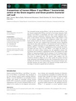
Full QCD simulation with a degenerate pair of up and down quarks and a strange quark with
a separate mass is often called N f = 2 + 1 QCD. In Fig. 1 we compare the computational cost of
N f = 2 + 1 QCD for the standard HMC algorithm estimated from (3.6) with the actual cost obtained
in our domain-decomposed HMC simulation at m π ≈ 300 MeV and 150 MeV. The figure demonstrates in a dramatic fashion that simulations of full lattice QCD at the physical point for light up,
down, and strange quarks are now reality.
The details of our mass-preconditioned domain-decomposed hybrid Monte Carlo algorithm are
spelled out in the Appendix of Ref. [7].

4.

Chiral behavior of hadron masses toward the physical point

We generated a set of configurations using the domain-decomposed HMC algorithm on the PACSCS massively parallel cluster computer. The up and down quarks are assumed degenerate with a
common hopping parameter κud and the strange quark hopping parameter κs is separate. The lattice
size is chosen to be 323 × 64 and the inverse bare gluon coupling constant β = 6/g 2 = 1.90. This
value corresponds to the lattice spacing a = 0.0907(13) fm. In Table 1 we list the run parameters.
We note that the run at (κud , κs ) = (0.137 00, 0.136 40) coincides with the lightest pion mass
with our previous attempt [46,47] based on the standard hybrid Monte Carlo algorithm. Thus we
have come down in the pion mass from m π ≈ 700 MeV to 150 MeV, which corresponds to a factor
(700/150)2 ≈ 22 reduction in the up-down quark mass.
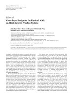
In Fig. 2 we show m 2π /m AWI
ud (for a definition of AWI quark mass, see Section 6), and the ratio of
pseudoscalar decay constants f K / f π . The almost linear behavior observed for heavier quark masses
(filled points) [46,47] is quite deceptive. The ratio m 2π /m AWI
ud bends upwards when the up-down quark
mass approaches the physical value shown by the vertical line. The ratio f K / f π , while not exhibiting
such dramatic behavior, nonetheless shows a clear upward deviation toward the experimental point.
Of course this is precisely the behavior expected from chiral perturbation theory toward vanishing
quark mass. It is clear, however, that without data close to the physical point, it would be, and in fact
it has been, very difficult to reliably pin down the value at the physical point from data in the heavy
quark mass region alone.
Given that calculations at the physical point are now possible, one should turn the tables and ask
if chiral perturbation theory correctly describes our data. We carry out such an analysis for the octet
10/31

Downloaded from at California Institute of Technology on July 3, 2015

Fig. 1. Simulation cost at m π ≈ 300 MeV by DDHMC (blue open circle) and m π ≈ 150 MeV by MPDDHMC
(blue closed circle) reproduced from Ref. [7] for 10 000 trajectories on a 323 × 64 lattice with a −1 ≈ 2 GeV.
The solid line indicates the cost estimate of N f = 2 + 1 QCD simulations with the standard HMC algorithm

at a = 0.1 fm with L = 3 fm for 100 independent configurations [36]. The vertical line denotes the physical
point. The sharp rise of the solid line toward the physical point has been dubbed the “Berlin Wall”.


PTEP 2012, 01A102

S. Aoki et al.

Table 1. Simulation parameters of our PACS-CS runs on a 323 × 64 lattice. Pion and kaon masses are
measured values multiplied by a −1 = 2.176 GeV as estimated in Ref. [7]. The third row lists the integers
(N0 , N1 , N2 , N3 , N4 ), specifying the multi-time steps. MD time is the number of trajectories multiplied
by the trajectory length τ . CPU time for unit τ using 256 nodes of PACS-CS is also listed.
κud
κs

0.137 00
0.136 40

0.137 27
0.136 40

0.137 54
0.136 40

0.137 54
0.136 60

0.137 70
0.136 40

0.137 81
0.136 40

0.137 785
0.136 60

m π (MeV)
m K (MeV)
τ

702
789
0.5
(4,4,10)
−
180
2000
0.29

570
713
0.5
(4,4,14)
−
180
2000
0.44

411
635

0.5
(4,4,20)
−
180
2250
1.3

385
582
0.5
(4,4,28)
−
220
2000
1.1

296
594
0.25
(4,4,16)
−
180
2000
2.7

154
553
0.25
(4,4,4,6)
0.9995

200
990
7.1

151
505
0.25
(4,4,2,4,4)
0.9995, 0.9900
220
2000
6.0

ρ
Npoly
MD time
CPU hour

of pseudoscalar mesons [7], and for the octet and decuplet of baryons [8]. Since we use the Wilsonclover quark action with explicit chiral symmetry breaking, we have to employ chiral perturbation
theory incorporating such breaking effects [62]. It turns out that these effects can be absorbed into the
leading order low energy constants so that the continuum expressions can be applied. If one assumes
that up, down, and strange quarks are light, then one should employ SU(3) chiral perturbation theory.
Taking the pion as an example, the well-known formula reads [63]
μη
2B0
m 2π
+ 2 (16m ud (2L 8 − L 5 ) + 16(2m ud + m s )(2L 6 − L 4 )) ,
= B0 1 + μπ −
2m ud
3

f0
f π = f 0 1 − 2μπ − μ K +

2B0
(8m ud L 5 + 8(2m ud + m s )L 4 ) ,
f 02

(4.1)

(4.2)

where
μPS =
m˜ 2π = 2m ud B0 ,

m˜ 2PS
1 m˜ 2PS
ln
16π 2 f 02
μ2

m˜ 2K = (m ud + m s )B0 ,

11/31

,

2
m˜ 2η = (m ud + 2m s )B0
3

(4.3)
(4.4)

Downloaded from at California Institute of Technology on July 3, 2015

Fig. 2. Comparison of the PACS-CS (red) [7] and the CP-PACS/JLQCD (black) [46,47] results for m 2π /m AWI
ud
(left) and f K / f π (right) as a function of m AWI
ud reproduced from Ref. [7]. Vertical line denotes the physical point
and star symbol represents the experimental value.


PTEP 2012, 01A102

S. Aoki et al.

Fig. 3. SU(2) chiral perturbation theory fit for m 2π /m AWI
ud and f K reproduced from Ref. [7]. FSE in legends
means including finite-size corrections. @ph means fit prediction at the physical point.

with μ the renormalization scale. There are six unknown low energy constants B0 , f 0 , L 4,5,6,8 in the
expressions above.
We simultaneously fit data to the formula such as the above for m 2π /(2m ud ), m 2K /(m ud + m s ), f π ,
and f K . We find that the fit exhibits a large χ 2 /dof, and the dependence on the strange quark mass
is not reproduced well. Furthermore, the next-to-leading order contribution coming from the kaon
loop is uncomfortably large in the decay constants.
A baryon spectrum analysis is tried using heavy baryon SU(3) chiral perturbation theory [64].
Incorporating the chiral symmetry breaking effects of the Wilson-clover quark action is left for future
work. The leading order formula yields a reasonable fit of the data. Including next-to-leading order

corrections, however, the flavor SU(3) coupling constants are found to take very small values quite
different from existing phenomenological estimates. It is our conclusion that the strange quark mass
is too large to be treated by chiral perturbation theory.
This situation leads us to make a reanalysis treating only up and down quarks as light. For this
purpose we use the SU(2) chiral perturbation theory formula, and make a linear extrapolation or
interpolation for the strange quark mass since our simulation points are close to its physical value.
We find good fits for pion masses below m π ≈ 400 MeV as shown in Fig. 3.
In Fig. 4 the light hadron spectrum extrapolated to the physical point using SU(2) chiral perturbation theory is compared with experimental values. Finite-size corrections are taken into account for
completeness, but they do not make large contributions. For the vector mesons and the baryons we
AWI . Data in the range m ≤ 400 MeV are
use a simple linear formula m had = αh + βh m AWI
π
ud + γh m s
used for these analyses.
12/31

Downloaded from at California Institute of Technology on July 3, 2015

Fig. 4. Light hadron spectrum extrapolated to the physical point using m π , m K and m as inputs reproduced
from Ref. [7]. The horizontal bars denote experimental values.


PTEP 2012, 01A102

S. Aoki et al.
Table 2. Meson and baryon masses at the physical point in
physical GeV units from Ref. [7]. m π , m K , m are the inputs.
Channel

Experiment

π
K
ρ
K∗
φ
N

Physical point

∗
∗

We need three physical inputs to determine the up-down and strange quark masses and the lattice
cutoff. We choose m π , m K , and m . The choice of m has both theoretical and practical advantages:
the baryon is stable in the strong interaction and its mass, being composed of three strange quarks,
is determined with good precision with small finite-size effects.
Numerical values are listed in Table 2. The largest discrepancy between our results and the experimental values is at most 3%, although errors are still not small for the ρ meson, the nucleon, and
the baryon. The results are clearly encouraging, but we have to note that we still need to remove
errors of O((a QCD )2 ).

5.

The reweighting technique and lattice QCD calculations at the physical point

Since reaching the physical point for light up, down, and strange quark masses has been achieved, we
may ask if it is possible to carry out calculations in lattice QCD precisely at the physical point. This
would be beautiful since, aside from effects of finite lattice spacing, one would be directly exploring
the physics of strong interactions as they take place in nature.
A priori we do not know the precise values of bare quark masses corresponding to the physical

point. Repeating simulations until one hits the physical point is clearly unattractive. The question,
therefore, is whether one can readjust the parameters to the physical point, given a set of configurations generated with parameters close to the physical point. The reweighting technique [55] turned
out to meet this need.
Let us consider evaluating O[U ](κud , κs ) (κ ,κs ) , which is the expectation value of a physical
ud
observable O at the target hopping parameters (κud , κs ), using the configuration samples generated
at the original hopping parameters (κud , κs ). We assume that ρud ≡ κud /κud 1 and ρs ≡ κs /κs 1.
The key is the following identity:

O[U ](κud , κs )

(κud ,κs )

=

DU O[U ](κud , κs )| det[Dκ [U ]]|2 det[Dκs [U ]]e−Sgluon [U ]
ud

DU | det[Dκ [U ]]|2 det[Dκs [U ]]e−Sgluon [U ]
ud

=

O[U ](κud , κs )Rud [U ]Rs [U ]
Rud [U ]Rs [U ] (κud ,κs )
13/31

(κud ,κs )

,

(5.1)

Downloaded from at California Institute of Technology on July 3, 2015

−
−
0.776(34)
0.896(9)
1.0084(40)
0.953(41)
1.092(20)
1.156(17)
1.304(10)
1.275(39)
1.430(23)
1.562(9)
−

0.1350
0.4976
0.7755
0.8960
1.0195
0.9396
1.1157
1.1926
1.3148
1.232
1.3837

1.5318
1.6725


PTEP 2012, 01A102

S. Aoki et al.

Fig. 5. Left: determination of the physical point on the (1/κud , 1/κs ) plane. Solid and open black circles denote
the original and target points, and crosses are the breakup points. Right: reweighting factors from the original
point to the target point plotted as a function of the plaquette value. Reproduced from Ref. [10].

Rud [U ] = | det W [U ](ρud )|2 , Rs [U ] = det W [U ](ρs )
W [U ](ρq ) ≡

Dκq [U ]
Dκq [U ]

= [ρq + (1 − ρq )Dκ−1 [U ]]−1
q

(5.2)
(5.3)

with ρq = κq /κq so that only Dκ−1 is needed to calculate W −1 .
q
The reweighting factors can be evaluated by a stochastic method. For the up and down quark sector,
for example, introducing a complex bosonic field η with color and spinor indices, the determinant of
W is expressed as
Rud [U ] = | det[W [U ](ρud )]|2

=

Dη† Dηe−|W

−1 [U ](ρ )η|2
ud

Dη† Dηe−|η|

= e−|W

2

−1 [U ](ρ )η|2 +|η|2
ud

η,

(5.4)

where · · · η means the expectation value with respect to η.
To reduce the fluctuations in the stochastic evaluation of Rud [U ] and Rs [U ] we employ the determinant breakup technique [66]. The interval between κq and κq is divided into N B subintervals:
κq ,κq + q , . . . , κq + (N B − 1) q , κq with q = (κq − κq )/N B , and the determinant ratios are
evaluated with the different set of η and multiplied together.
We implement the reweighting procedure in the following way. Since the lightest pion mass
m π ≈ 150 MeV and the lightest kaon mass m K ≈ 550 MeV reached in the first round of simulations [7] are still heavier than the physical values by about 10%, we make an additional
run at (κud , κs ) = (0.137 785, 0.136 60). With preliminary trial runs, we then estimate (κud , κs ) =
(0.137 796 25, 0.136 633 75) as the target for the physical point. The reweighting is carried out with
N B = 3 steps for both κud and κs , adding one more step going beyond the target value in the κs
direction.

In the left-hand of panel of Fig. 5 we show how we reach the target point (open circle) from the
original point (filled circle) through a grid of breakup points. In the right-hand panel of the same
figure are shown the reweighting factors from the original to the target points calculated for a set
of 80 configurations as a function of plaquette value. The points are distributed within an order of
magnitude around the value unity, demonstrating that the fluctuation of the reweighting factors is
14/31

Downloaded from at California Institute of Technology on July 3, 2015

where


PTEP 2012, 01A102

S. Aoki et al.

Fig. 6. Hadron masses normalized by m in comparison with experimental values reproduced from Ref. [10].
The target result for the ρ meson is below the figure.

6.

Strong coupling constant and quark masses—fundamental constants of QCD

The values of the strong coupling constant αs = g 2 /4π and the quark masses m q , q = ud, s are
fundamental constants of nature. Since they both vary under scale change, we need to understand
their renormalization, and specify the scale μ and the scheme to quote their values. We employ the
finite-volume Schrödinger functional method for this purpose [67,68].

6.1.

Strong coupling constant

The Schrödinger functional is the partition function defined on a lattice of a finite extent L 3 × T with
certain boundary conditions imposed on the gluon and quark fields. The coupling constant g¯ 2 (L) in
the Schrödinger functional scheme is defined through a variation of the effective action under a
certain change of the gluon boundary condition.
The fundamental quantity in this method is the step scaling function σ (u). It represents the
change of the coupling constant under a scale change by some factor s, typically taken to be s = 2;
g¯ 2 (s L) = σ (u) with u = g¯ 2 (L). One numerically calculates the lattice value of the step scaling function (u, a/L) for a set of lattice sizes and the bare coupling constant, and takes the limit a/L → 0 to
find the continuum limit σ (u) = lima/L→0 (u, a/L). This is done for a set of values of u covering
a sufficient range from weak to strong coupling. Once one has σ (u), one can calculate the β function
√
√
√ √
√
β( u) = −L∂ g¯ 2 (L)/∂ L/2 u recursively through β( σ (u)) = β( u) u/σ (u)∂σ (u)/∂u.
In Fig. 7 we plot our results for the step scaling function (left-hand panel) and the beta function
(right-hand panel) for N f = 3 QCD in the Schrödinger functional scheme [9].
The strong coupling constant αs (μ) is usually quoted in the MS scheme at a high energy scale
for
μ = M Z . Finding this value requires evaluating the renormalization-group invariant scale
N f = 3 QCD at low energy, and then running up to M Z , crossing the charm and bottom thresholds on the way. Since we have the step scaling function, the first step can be carried out if we have
the value of the coupling constant g¯ 2 (L max ) at some scale L max . This in turn requires the value of
15/31

Downloaded from at California Institute of Technology on July 3, 2015

under control. In addition, we observe a clear positive correlation between the reweighting factors
and the plaquette value as expected.
In Fig. 6 we plot the hadron masses calculated at the target point normalized by that of in comparison with experiment. Matching to the physical point is very good. The deviation for the ρ meson

may be ascribed to its resonance nature, and those for baryons probably reflect finite-size effects; the
box size of 3 fm for our 323 × 64 lattice is probably too small for baryons.


PTEP 2012, 01A102

S. Aoki et al.

L max in physical units, which we supply from the determination of the lattice spacing through hadron
mass spectrum calculations.
In order to control the continuum limit, we may employ the scale determination from the previous
N f = 2 + 1 QCD simulation at three lattice spacings [46,47] carried out by the joint CP-PACSJLQCD Collaboration using the same gluon and quark actions. The result is given by [9]
αs (M Z ) = 0.12047(81)(48)(+0
−173 ),
(5)
MS

= 239(10)(6)(+0
−22 ) MeV,

(6.1)
(6.2)

where the first error is statistical and the second represents the systematic error of perturbative
matching across the charm and bottom thresholds. The last parenthesis shows an estimate of the
systematic error from a constant and a linear continuum extrapolation. For comparison, the world
average excluding lattice results is αs (M Z ) = 0.1186(11). [70]
We have to note that the above results do not include systematic errors due to chiral extrapolation. If
one uses the scale from the current N f = 2 + 1 runs using the domain-decomposed HMC algorithm
(5)

down to m π ≈ 150 MeV [7], one finds αs (M Z ) = 0.1225(14)(5) and MS = 266(20)(7) MeV,
where the meanings of the errors are the same as the first two in (6.1).

6.2.

Light quark masses

We define the bare quark mass through the axial vector Ward–Takahashi identity (AWI) by taking
the ratio of matrix elements of the pseudoscalar density P = qγ
¯ 5 q and the fourth component of the
axial vector current A4 :
imp
0|∇4 A4 |PS
AWI
AWI
,
(6.3)
m¯ f + m¯ g =
0|P|P S
where |PS denotes the pseudoscalar meson state at rest and f and g ( f, g = u, d, s) label the flavors
imp
of the valence quarks. We employ the non-perturbatively O(a)-improved axial vector current A4 =
A4 + c A ∇¯ 4 P with ∇¯ 4 the symmetric lattice derivative, and c A = −0.03876106 as determined in
Ref. [71]. The O(m q a) corrections are removed by defining
1 + bA
m AWI
=
f

m VWI

f
u0

m VWI
1 + b P uf 0

16/31

m¯ AWI
f ,

(6.4)

Downloaded from at California Institute of Technology on July 3, 2015

Fig. 7. Left: step scaling function σ (u)/u with u = g¯ 2 (L) for N f = 3 QCD. The dotted line represents the
three-loop perturbative result. The solid line is a polynomial fit of the step scaling function. Right: β-function
of QCD for N f = 3 and 2. The solid lines are three-loop perturbative results for comparison. Data for N f = 2
are reproduced from Ref. [69]. Reproduced from Ref. [9].


PTEP 2012, 01A102

S. Aoki et al.

where the improvement coefficients b A,P are perturbatively evaluated up to the one-loop level [72]
with tadpole improvement.
The renormalization of quark mass as defined above is given by those of Aμ and P. We therefore
have to determine the step scaling function of the pseudoscalar density σ P (u), and the renormalization constant Z A for the axial vector current which is scale independent due to partial
conservation.

In Fig. 8 we show our results for the step scaling function for the pseudoscalar density and the
renormalization constant for the axial vector current. We combine them with the bare quark masses
determined in hadron mass spectrum calculations to calculate the quark masses m q (μ) at a scale μ in
physical units. With the present PACS-CS data [7], we find m MS
ud (μ = 2 GeV) = 2.78(27) MeV for
MS
the average up and down quark, and m s (μ = 2 GeV) = 86.7(2.3) MeV for the strange quark [11].
We have to wait until simulations at weaker couplings are made to see if these values stay toward the
continuum limit.

7.

Resonance properties through finite-volume two-particle analyses

Masses of resonances such as ρ, K ∗ and cannot be correctly extracted from the exponential decay
of two-point functions. Instead, one can use the relation between the energies of two-particle states
on a finite box and the elastic phase shift to calculate the latter, from which one can extract the pole
position and the resonance width. While the theoretical foundations of this topic were laid out quite
early [26,27] and have been explored in simulations for many years [73,74], it is only recently, with
the development of full QCD simulations near the physical point, that a realistic calculation of the
resonance properties has become feasible.
The basis is the formula which connects the energy E of a two-particle state on a finite box with
the elastic phase shift δ(k) in the same channel. When the two particles are degenerate in mass, k is
√
defined by E = 2 m 2 + k 2 with m the mass of each particle. For zero center of mass momentum
and a spatial lattice of a size L 3 , the connection is given by
1
1
= 3/2 Z 00 (1, q),
tan δ(k)

π q

(n2 − q 2 )−s

Z 00 (s, q) =
n∈Z 3

with q = k L/(2π ). The extension to a non-zero center of mass is also known [75].
17/31

(7.1)

Downloaded from at California Institute of Technology on July 3, 2015

Fig. 8. Left: step scaling function σ P (u) with u = g¯ 2 (L) for the pseudoscalar density for N f = 3 QCD. The
dotted line represents the two-loop perturbative result. The solid line is a polynomial fit of the step scaling function. Right: β dependence of Z A (g0 ). Red filled circles are our non-perturbative renormalization factor. The
solid line is a perturbative result at one loop. Stars are from tadpole-improved perturbation theory. Reproduced
from Ref. [11].


PTEP 2012, 01A102

S. Aoki et al.

Table 3. The ground and first exited states with isospin (I, Iz ) = (1, 0) for the irreducible representations
considered in Ref. [15], ignoring hadron interactions. P is the total momentum, g is the rotational group on the
lattice in each momentum frame and is the irreducible representation of the group. The vectors in parentheses
after (π π ) and ρ refer to the momenta of the two pions and the ρ meson in units of 2π/L. We use the notation
(π π )(p1 )(p2 ) = π + (p1 )π − (p2 ) − π − (p1 )π + (p2 ) for two-pion states. Index j for the T−
1 representation takes

j = 1, 2, 3 and k for E− takes k = 1, 2.
Frame

PL/(2π )

g

CMF
MF1
MF1
MF2

(0, 0, 0)
(0, 0, 1)
(0, 0, 1)
(1, 1, 0)

Oh
D4h
D4h
D2h

T−
1
E−
A−
2
B−
1

ρ j (0)
ρk (0, 0, 1)
ρ3 (0, 0, 1)
(ρ1 + ρ2 )(1, 1, 0)

(π π )(e j )(−e j )
(π π )(e3 + ek )(−ek ) − (π π )(e3 − ek )(ek )
(π π )(0, 0, 1)(0, 0, 0)
(π π )(1, 1, 0)(0, 0, 0)

G(t) =

0|(π π )† (t)(π π )(ts ) |0
0|ρ † (t)(π π )(ts )|0

0|(π π )† (t)ρ(ts )|0
0|ρ † (t) ρ(ts )|0

.

(7.2)

We extract the ground and first excited state energies by a single exponential fit of the two eigenvalues
λ1 (t) and λ2 (t) of the matrix M(t) = G(t)G −1 (t R ) with some reference time t R , assuming that the
lower two states dominate the time correlation function.
√
In Fig. 9 we plot the results for the phase shift in terms of k 3 /( s tan δ(k)). For an effective ρπ π
coupling of form L eff = gρπ π μabc abc (k1 − k2 )μ ρμa ( p)π b (k1 )π c (k2 ), we expect a linear relation
given by
√

k3
6π
/ s = 2 (m 2ρ − s).
(7.3)
tan δ(k)
gρπ π
A χ 2 fit then yields an estimate of the resonance mass m ρ and the ρπ π coupling gρπ π . We list the
results in Table 4.
In terms of gρπ π , the physical ρ meson width is given by
ρ

=

2
3
gρπ
π k
6π m ρ

(7.4)

where k = m 2ρ /4 − m 2π and physical values should be used for m ρ and m π . Substituting the experimental width ρ = 146.2(7) MeV yields gρπ π = 5.874(14). Our results at the two pion masses
18/31

Downloaded from at California Institute of Technology on July 3, 2015

We apply this formalism to the two-pion channel to extract the I = 1 P-wave phase shift, with
which we calculate the resonance properties of the ρ meson [15]. Calculations are carried out for the
two configuration sets corresponding to m π = 410 MeV and 300 MeV on a 323 × 64 lattice listed in
Table 1.

In order to calculate the phase shift at various energies from configurations with a single size,
we consider three choices for the total momentum: the center of mass frame with total momentum P = (0, 0, 0) (CMF), the non-zero momentum frame with P = (2π/L)(0, 0, 1) (MF1), and
P = (2π/L)(1, 1, 0) (MF2). The ground and first excited states for these momenta with isospin
(I, Iz ) = (1, 0), ignoring the hadron interactions, are shown in Table 3 where g is the rotational group
in each momentum frame on the lattice and is the irreducible representation of the rotational group.
√
−
s = E 2 − P2 for the two-pion state is
For the T−
1 and E representations the invariant mass
sufficiently heavier than the ρ mass so that we only calculate the ground state energy from the ρ
−
meson propagator in the standard way. For the A−
2 and B1 representations for which the invariant
mass is close to or lighter than the ρ mass, we calculate a 2 × 2 matrix of correlation functions in
the ρ and π π channels given by


PTEP 2012, 01A102

S. Aoki et al.

Table 4. The ρ resonance mass and ρπ π coupling
gρππ estimated at the pion mass in the first row.
mπ
410 MeV
300 MeV

mρ

gρππ

892.8(5.5)(13) MeV
863(23)(12) MeV

5.52(40)
5.98(56)

m π = 410 MeV and 300 MeV, although not close enough to the physical point, are reasonably
consistent with it.

8.

Pion electromagnetic form factor

The electromagnetic form factor of a pion is defined by
π + ( p )|Jμ |π + ( p) = ( pμ + pμ )G π (Q 2 ),

(8.1)

where Q 2 = −q 2 = −( p − p)2 is the four-momentum transfer, and Jμ is the electromagnetic
current given by
2
1¯
1
¯ μ u − dγ
(8.2)
Jμ = uγ
μ d − s¯ γμ s.
3

3
3
An interesting feature is that the slope of the form factor at the origin, i.e., the electromagnetic charge
radius, defined by
dG π (q 2 )
r2 = 6
|q 2 =0 ,
(8.3)
dq 2
is expected to diverge logarithmically as m π becomes small.
To extract the form factor, we use the ratio defined by
R(τ ) =

C 3pt ( p , t f ; p, 0; τ )
.
C 3pt ( p , t f ; p , 0; τ )

(8.4)

where
C 3pt ( p , t f ; p, 0; τ ) = π + ( p , t f )Jμ (τ )π + ( p, 0) ,

(8.5)

is the pion-to-current three-point function. If one chooses the momenta of the two pions satisfying
p = p but | p | = | p|, the ratio converges for large τ and t f as
R(τ ) →

2
G bare

π (Q )
= G π (Q 2 ).
G bare
(0)
π

19/31

(8.6)

Downloaded from at California Institute of Technology on July 3, 2015

√
Fig. 9. k 3 /( s · tan δ(k)) as a function of the square of the invariant mass s at m π = 410 MeV (left) and
m π = 300 MeV (right) reproduced from Ref. [15]. The same symbols for four representations are used in both
−
panels. The dotted lines are finite-size formulas for the A−
2 and B1 representations. The solid line for each
quark mass is the fit to (7.3).


PTEP 2012, 01A102

S. Aoki et al.

In contrast with more conventional choices of momenta such as p = 0 and p = 0, our ratio does
not involve the two-point function of the pion, and this leads to much better signals as the pion mass
is decreased [13].
On a 323 × 64 lattice with a 2 GeV inverse lattice spacing, the minimum non-zero quark momentum for the periodic boundary condition 2π/La is about 0.4 GeV. In order to study the form factor
for smaller momentum transfer, we use the partially twisted boundary condition technique [76]. If

one imposes the following boundary condition on valence quark fields:
q(x + Le j ) = e2πiθ j q(x),

j = 1, 2, 3,

(8.7)

the spatial momentum of that quark is quantized according to
pj =

2π θ j
2π n j
+
,
L
L

j = 1, 2, 3,

(8.8)

where L denotes the spatial lattice size, e j the unit vector in the spatial jth direction, and θ j a real
parameter. In this way one can explore arbitrarily small momenta on the lattice by adjusting the
value of twist θ j . We apply the Z (2) ⊗ Z (2) random noisy source to improve on statistical errors, as
introduced in Ref. [77].
In the left-hand panel of Fig. 10, we plot our result [13] for the form factor at m π ≈ 300 MeV and
410 MeV as a function of the momentum transfer Q 2 . The dashed and solid lines are data fits of the
next to next leading order (NNLO) formula of the form factor to SU (2) chiral perturbation theory,
combining data for m π = 300 MeV and 410 MeV.
In the right-hand panel we shown the charge radius calculated from the NNLO chiral perturbation

theory fit (open circles) as compared to experiment at the physical point (red filled circle). Blue filled
circles are the results of the monopole fit of form
G π (Q 2 ) =

1
1+

2
Q 2 /Mmono

.

(8.9)

We see that chiral perturbation theory is reasonably convergent over the range m π ≈ 300 − 410 MeV
and Q 2 ≤ 0.1 GeV2 explored in this calculation. The charge radius extrapolated to the physical point
is in agreement with experiment, albeit with a 10% error.
The PACS-CS gauge configurations have a set corresponding to m π ≈ 150 MeV. We tried to calculate the form factor on this set, and found that the pion two- and three-point functions exhibited
20/31

Downloaded from at California Institute of Technology on July 3, 2015

Fig. 10. Left: pion form factor and NNLO SU(2) chiral fits using the decay constant f π measured at each m π
and combining data at m π = 296 MeV and 411 MeV. Right: charge radius, with filled circles from monopole
fits, and open circles from NNLO SU(2) chiral fits. Upward triangles and downward triangles are NLO and
NNLO contributions, respectively. Reproduced from Ref. [13].


PTEP 2012, 01A102

S. Aoki et al.

very large fluctuations, to the extent that taking a meaningful statistical average was difficult. This
trend became more pronounced as the twist carried by quarks was made larger. Since Lm π ≈ 2.3 at
this pion mass for L = 32, we suspect that this phenomenon is caused by the small size of the lattice
relative to the pion mass, and the consequent increase in large fluctuations. It is our conclusion that
calculating the pion form factor directly at the physical point requires larger lattices such as 644 .

9.

Heavy quark physics on a physical light quark sea

Q¯ x Dx,y Q y ,

SQ =

(9.1)

x,y
†

Dx,y = δx y − κ Q

[(rs − νγi )Ux,i δx+i,y
ˆ + (rs + νγi )U x,i δx,y+iˆ ]
i
†

− κ Q [(rt − νγi )Ux,4 δx+4,y
ˆ + (rt + νγi )U x,4 δx,y+4ˆ ]

⎡
⎤
− κ Q ⎣c B

Fi4 (x)σi4 ⎦ ,

Fi j (x)σi j + c E
i, j

(9.2)

i

where κ Q is the hopping parameter for the heavy quark. In the present calculation we adjust
the parameters rt , rs , c B , c E and ν as follows. We are allowed to choose rt = 1, and we employ
the one-loop perturbative value for rs [79]. For the clover coefficients c B and c E we include the
NP for three-flavor dynamical QCD [57], and calnon-perturbative contribution in the massless limit cSW
culate the heavy quark mass dependent contribution perturbatively to one-loop order [79] according
to
NP
.
c B,E = (c B,E (m Q a) − c B,E (0))PT + cSW

(9.3)

The parameter ν is determined non-perturbatively to reproduce the relativistic dispersion relation for
the spin-averaged 1S states of charmonium. Writing
2
E( p)2 = E(0)2 + ceff
| p|2 ,

(9.4)

√
for | p| = 0, 1, 2, and demanding the effective speed of light ceff to be unity, we find ν = 1.1450511,
with which we have ceff = 1.002(4). The remaining cutoff errors are αs2 f (m Q a)(a QCD ), instead
21/31

Downloaded from at California Institute of Technology on July 3, 2015

We have seen in Section 5 that the reweighting technique allows us to adjust the light up, down,
and strange quark masses to the physical values. We can therefore explore heavy quark physics
on a physical light quark sea background. This has the advantage that systematic errors associated
with chiral extrapolation in the light quark masses, which otherwise plague physical predictions, are
absent. Errors due to charm and bottom quenching are expected to be small. We apply this method
to the charm quark for the set of configurations at (κud , κs ) = (0.137 785, 0.136 60) reweighted to
(0.137 796 25, 0.136 633 75).
Since the lattice spacing on our set of configurations is a −1 ≈ 2 GeV, the charm quark can be
treated directly, i.e., without resorting to heavy quark effective theory. We employ the relativistic
heavy quark formalism [78] to deal with the discretization errors of O(m charm a).
The relativistic heavy quark formalism is designed to reduce the cutoff errors of O((m Q a)n ) with
arbitrary order n to O( f (m Q a)(a QCD )2 ), where f (m Q a) is an analytic function around the massless point m Q a = 0, once all of the parameters in the relativistic heavy quark action have been
determined non-perturbatively. The action is given by


PTEP 2012, 01A102

S. Aoki et al.

Fig. 11. Left: charmonium mass spectrum in N f = 2 + 1 lattice QCD normalized by the experimental values

reproduced from Ref. [14]. Right: hyperfine splitting of charmonium calculated with different numbers of
dynamical light flavors, Ref. [14] for N f = 2 + 1 and Ref. [14] for N f = 2, 0.

M(1S) = (Mηc + 3M J/ψ )/4 = 3.0678(6) GeV.

(9.5)

This leads to κcharm = 0.109 599 47 for which our lattice measurements yield the value M(1S)lat =
3.067(1)(14) GeV, where the first error is statistical, and the second is a systematic error from the
scale determination.
The charm quark mass is calculated from the bare value m AWI
charm obtained from the PCAC relation
and the renormalization factor Z m (μ). Similar to the clover coefficients, the renormalization factor
is estimated by combining the non-perturbative value at the massless point from the Schrödinger
functional method and the charm quark mass dependent piece in one-loop perturbation theory. The
result is given by
MS
m MS
charm (μ = m charm , N f = 4 running) = 1.249(1)(6)(35) GeV,

(9.6)

where the first error is statistical, the second is systematic from the scale determination, and the third
from uncertainties in the renormalization factors.
We show in the left-hand panel in Fig. 11 the charmonium spectrum normalized by experiment. The
agreement is satisfactory within one standard deviation. The right-hand panel demonstrates that light
dynamical sea quark effects are crucial for understanding charmonium hyperfine splitting. The filled
circle shows the result from PACS-CS [14]. Results with dynamical up and down quarks (N f = 2)
and with the quenched approximation (N f = 0) are from the CP-PACS Collaboration [80] using the
same heavy quark formalism. A small discrepancy that is still visible between the filled circle and

experiment should go away as we approach the continuum limit.
The decay constants f D and f Ds of charmed D and Ds mesons are important for determining the
Vcd and Vcs elements of the Cabibbo–Kobayashi–Maskawa matrix since they are directly related to
the leptonic decay width
m l2
G 2F 2
2
m mD fD 1 − 2
(D → lν) =
8π l
mD
22/31

2

|Vcd |2 .

(9.7)

Downloaded from at California Institute of Technology on July 3, 2015

of f (m Q a)(a QCD )2 , due to the use of one-loop perturbative values in part for the parameters of
our heavy quark action.
We tune the heavy quark hopping parameter by the mass for the spin-averaged 1S states of
charmonium, experimentally given by [65]


PTEP 2012, 01A102

S. Aoki et al.

Table 5. Results for the decay constants of the D and Ds
mesons from Ref. [14]. The first error is statistical, the second is a systematic error from the scale determination, and
the third is from the renormalization factor. Experimental
data are also listed [65].
f D (MeV)
f Ds (MeV)
f Ds / f D

Lattice

Experiment

226(6)(1)(5)
257(2)(1)(5)
1.14(3)(0)(0)

206.7(8.9)
257.5(6.1)
1.25(6)

10.

QCD + QED simulation and electromagnetic mass splitting of hadron masses

Up to now we have assumed isospin symmetry in the quark mass, m u = m d . However, in nature,
isospin symmetry is broken by the quark mass difference, m u = m d , and by the difference of the quark
electric charges, eu = ed . Isospin symmetry breaking causes mass splittings in isospin multiplets
of light hadrons, e.g., m K 0 − m K ± , m n − m p . The magnitude of the splittings is not large, but is
important since, e.g., it is this difference which guarantees the stability of the proton. Thus, our next
target should be a QCD + QED lattice calculation at the physical point incorporating quark mass

differences.
A pioneering QCD + QED lattice simulation was carried out a long time ago [83,84] using the
quenched approximation both for QCD and QED. The possibility of including dynamical QED
effects was first investigated in Ref. [85]. Recently, results for the low-energy constants in chiral perturbation theory including dynamical quark effects both in QCD and QED were reported [86]. We
present our results for a full QCD + full QED simulation at the physical point using the reweighting
technique [17,18].
Let D(e, κ) be the Wilson-clover operator for electric charge e and hopping parameter κ on a
background gluon field Unμ and U (1) electromagnetic field Uem nμ . The reweighting factor we have
to calculate is given by
D(eu , κu∗ ) D(ed , κd∗ ) D(es , κs∗ )
,
det
D(0, κud ) D(0, κud ) D(0, κs )

(10.1)

∗
where eu,d,s and κu,d,s
are the physical charge and hopping parameter of up, down, and strange quarks.
Controlling the fluctuations of the reweighting factor turned out to be more difficult than the pure
QCD case treated in Section 5. First, the reweighting factor for each flavor has a significant fluctuating O(e) part. This problem was tamed by estimating the reweighting factor for the three flavors
together, the reason being the fact that the total charge vanishes as eu + ed + es = 0 [86]. Secondly,
for the Wilson-clover quark action, the additive quark mass renormalization due to short-distance

23/31

Downloaded from at California Institute of Technology on July 3, 2015

Our results are compared with experiment in Table 5. While the agreement for f Ds is satisfactory,
the result for f D differs by about two standard deviations. It is necessary to take the continuum limit

for a definite comparison.
With the CLEO value of (D → lν) [81,82], we obtain |Vcd |(lattice) = 0.205(6)(1)(5)(9), where
the first error is statistical, the second is systematic due to the scale determination, the third is
uncertainty in the renormalization factor, and the fourth represents the experimental error of the leptonic decay width. Similarly, using the CLEO value of (Ds → lν) [81,82], we find |Vcs |(lattice) =
1.00(1)(1)(3)(3).


PTEP 2012, 01A102

S. Aoki et al.

Table 6. Comparison of masses calculated in QCD + QED and experiment from Ref. [17,18]. Lattice spacing
a −1 = 2.235(11) GeV is fixed by the − baryon mass.
QCD + QED
Experiment

m π + (MeV)

m K + (MeV)

m K 0 (MeV)

m

137.7(8.0)
139.570 18(35)

492.3(4.7)
493.677(16)

497.4(3.7)
497.614(24)

input
1672.45(29)

−

(MeV)

QED effects turned out to be quite large. This difficulty was treated by generating the U (1) electromagnetic field on a lattice twice as fine as the original QCD lattice and blocking over 24 sublattices
to smooth out short distance fluctuations. We also applied a large number of breakups.
In practice, we start from the set of configurations at (κud , κs ) = (0.137 785, 0.136 60) on
a 323 × 64 lattice and reweight to (κu∗ , κd∗ , κs∗ ) = (0.137 870 14, 0.137 797 00, 0.136 695 10) and
√
(eu , ed , es ) = (2/3, −1/3, −1/3)ephys with ephys = 4π/137. We use 400 breakups for QED and 26
for QCD with 12 noise sources for each breakup on 80 configurations. The target hopping parameters
are tuned to reproduce the masses of the π + , K + , and K 0 mesons and the − baryon.
In Table 6 we use the − baryon mass to fix the lattice spacing a −1 and compare the calculated
π + , K + , K 0 masses with experimental values; this demonstrates that we have successfully tuned the
hopping parameter taking into account full QCD and QED effects.
Figure 12 shows the ratio of K 0 to K + propagators whose time dependence is expected to follow
K 0 (t)K 0 (0)
K + (t)K + (0)

Z (1 − (m K 0 − m K + )t),

(10.2)

where we assume (m K 0 − m K + )t

1. The negative slope indicates m K 0 > m K + . The fit result
with [tmin , tmax ] = [13, 30] gives 4.54(1.09) MeV, which is consistent with the experimental value
3.937(28) MeV [65] within error.
In Table 7 we list the quark masses in the MS scheme at scale μ = 2 GeV. Non-perturbative renormalization factors employed for the pure QCD case are also used here [11]. The QED corrections to
the renormalization factor, whose contribution would be a level of 1% or less, are ignored. The first
errors are statistical and the second ones are associated with computation of the non-perturbative
normalization factors. Finite-size corrections due to QED, if estimated with chiral perturbation theory [87], would be −13.50%, +2.48%, and −0.07% for the up, down, and strange quark masses,
respectively.
24/31

Downloaded from at California Institute of Technology on July 3, 2015

Fig. 12. Ratio of K 0 to K + propagators to detect the mass difference m K 0 − m K + reproduced from Ref. [17,18].
Our results (black symbols) are consistent with the expected slope from the experimental value of m K 0 − m K +
(red line).


PTEP 2012, 01A102

S. Aoki et al.

Table 7. Quark masses calculated in QCD + QED [17,18]. Lattice spacing is fixed by the

−

baryon mass.

m u (MeV)

m d (MeV)

m s (MeV)

m ud (MeV)

m u /m d

m s /m ud

2.57(26)(7)

3.68(29)(10)

83.60(58)(2.23)

3.21(24)(8)

0.699(51)

26.7(2.0)

11.

Going beyond hadrons to nuclei

11.1.

Deuteron

The simplest nucleus is the two-nucleon system which includes deuteron. The dynamics for this

system, however, is already subtle; the binding in the spin triplet deuteron channel is quite shallow
and the spin singlet state is not bound. Lattice studies of the two-nucleon system were started quite
some time ago [89,90], and have been addressed extensively, including recent simulations in full
QCD with dynamical quarks. Nonetheless, no clear evidence of bound state formation has been
reported so far. Indeed, all studies analyzed data based on the assumption that bound states do not
form for heavy pions beyond m π 0.3 GeV, and tried to extract the scattering lengths using Lüscher’s
formula [26,27] relating two-particle energies to elastic scattering data.
Clarifying this first issue requires a systematic finite-size study of the energy levels of the twonucleon system. Our strategy is: (i) resort back to quenched QCD to access a large range of spatial
lattice sizes from L = 3 fm to 12 fm with high statistics, (ii) initially work with a heavy quark
mass, and (iii) in addition to the standard single-state analysis looking for the lowest energy for
the two-particle ground state, carry out a two-state analysis for the ground and first excited states
diagonalizing the 2 × 2 matrix of the nuclear Green’s function. The last point is important to confirm the bound state nature since, as is well known from quantum mechanics, a shallow bound state
is accompanied by a scattering state just above the two-particle threshold in a finite volume. In this
analysis we employ the Helmholtz kernel for the sink operator given by
Wq 2 (r ) = Cq 2
n∈Z3

ei(2π/L)n·r
,
n2 − q 2

(11.1)

where q 2 is a parameter, r is the relative coordinate between two nucleons, and the overall factor Cq 2
is determined from the normalization condition |Wq 2 (rmax )| = 1.
The calculations are made in quenched QCD with the renormalization-group improved Iwasaki
gluon action at β = 2.416, which corresponds to the lattice spacing a −1 = 1.541 GeV as determined
from the Sommer scale r0 = 0.49 fm. The Wilson-clover quark action with the tadpole-improved
clover term is used. The nucleon and pion masses are m N = 1.617 GeV and m π = 0.800 GeV. The
25/31

Downloaded from at California Institute of Technology on July 3, 2015

The strong interaction dynamically generates a hierarchical structure: three quarks are bound to form
a nucleon with an energy of 1 GeV, and nucleons are bound to form atomic nuclei with a binding
energy of about 10 MeV per nucleon. Since all nuclei are ultimately made of quarks and gluons,
lattice QCD should help us quantitatively understand the structure and property of known nuclei
based on its first principles. This direct approach will be more important and indispensable if we are
to extract reliable predictions for experimentally unknown nuclei in the neutron-rich region of the
nuclear chart.
Two approaches are being pursued in this direction; one can extract nuclear potentials from lattice
QCD calculations and use them as input in nuclear physics calculations [88], or one can calculate
nuclear observables directly in lattice QCD [12,16]. We describe here two attempts of the latter
category.