DSpace at VNU: Using weighted dynamic range for histogram equalization to improve the image contrast

Huynh-The et al. EURASIP Journal on Image and Video Processing 2014, 2014:44
/>
R ESEA R CH

Open Access

Using weighted dynamic range for histogram
equalization to improve the image contrast
Thien Huynh-The1† , Ba-Vui Le1† , Sungyoung Lee1* , Thuong Le-Tien2 and Yongik Yoon3

Abstract
In this paper, an effective method, named the brightness preserving weighted dynamic range histogram equalization
(BPWDRHE), is proposed for contrast enhancement. Although histogram equalization (HE) is a universal method, it is
not suitable for consumer electronic products because this method cannot preserve the overall brightness. Therefore,
the output images have an unnatural looking and more visual artifacts. An extension of the approach based on the
brightness preserving bi-histogram equalization method, the BPWDRHE used the weighted within-class variance
as the novel algorithm in separating an original histogram. Unlike others using the average or the median of gray
levels, the proposed method determined gray-scale values as break points based on the within-class variance to
minimize the total squared error of each sub-histogram corresponding to the brightness shift when equalizing them
independently. As a result, the contrast of both overall image and local details was enhanced adequately. The
experimental results are presented and compared to other brightness preserving methods.
Keywords: Contrast enhancement; Weighted dynamic range; Brightness preserving; Within-class variance

Introduction
Enhancing contrast of images by using histogram equalization (HE) is the standard technique to improve the
visual image by stretching the narrow input image histogram [1]. However, it is not the appropriate method
for consumer electronics, such as TV, because it changes
the brightness of the original image strongly and degrades
the image quality in visualization. Various methods
have been proposed to limit the level of enhancement
based on modifying the input histogram with mapping

functions. The brightness preserving bi-histogram equalization (BBHE) [2], the dualistic sub-image histogram
equalization (DSIHE) [3], and the minimum mean brightness error bi-histogram equalization (MMBEBHE) [4]
divided the input histogram into two sub-histograms by
a separating point. In order to enhance the image contrast, each sub-histogram was equalized independently.
The BBHE method used the gray level as the mean value
of image brightness to separate an input histogram into
two parts: the first one is from the minimum gray level
*Correspondence:
† Equal contributors
1 Department of Computer Engineering, Kyung Hee University, 1732
Deokyoungdae-ro, Giheng-gu, Youngin-si, Seoul, Gyeonggi-do 446-701, Korea
Full list of author information is available at the end of the article

to the mean, and the second one is from the mean to
the maximum gray level. The DSIHE method also used
a similar approach to enhance the image contrast, except
applying the median value instead of the mean value. In
practice, the DSIHE is better than the BBHE in both preserving the image brightness and conserving the information content. The simple method to find out the separated
point is to test all possible gray-scale values from 0 to L−1
of the histogram by calculating the difference between
the mean brightness of input and the mean brightness of
output. The separated point is chosen as the value that
achieves the minimum difference in overall brightness.
Although the above methods are better than HE in keeping the brightness of images, the visualization of enhanced
images is degraded seriously, sometimes in detail and
overall.
Based on the BBHE, the recursive mean separate histogram equalization (RMSHE) [5] and the recursive subimage histogram equalization (RSIHE) [6] divided an
original histogram into 2n sub-histograms, where n is a
positive integer value. The RMSHE splits the histogram
into two parts by using the average of input brightness

before separating one more time for each sub-histogram
to have four segments in total. In practice, there are 2n
sub-histograms for n separated times. Having the same

© 2014 Huynh-The et al.; licensee Springer. This is an Open Access article distributed under the terms of the Creative Commons
Attribution License ( which permits unrestricted use, distribution, and reproduction
in any medium, provided the original work is properly credited.


Huynh-The et al. EURASIP Journal on Image and Video Processing 2014, 2014:44
/>
idea with the RMSHE in separation of more segments,
the RSIHE also divided the histogram as well based on
the median, rather than the mean of intensity values. Of
note in these approaches, the output image looks like
the copy version of the input image when n is too large,
i.e., there is clearly no contrast enhancement here. In [7],
the brightness preserving dynamic histogram equalization
(BPDHE) divided the input histogram into an arbitrary
number of sub-histograms based on break points which
were determined by the local minima of the histogram.
Based on the total number of pixels contained in each
sub-histogram, the new partitions are obtained from the
dynamic ranges by the new function for resizing. After
the histogram equalization step, the output image would
be normalized in brightness with the original to ensure
that the mean of output intensity is close to the mean of
input intensity. Moreover, the authors in [8] proposed a
contrast enhancement method using the dynamic range
separate histogram equalization (DRSHE) approach to

preserve the naturalness of images and improve the overall
contrast. The weighted average of absolute color difference (WAAD) used in the DRSHE produced an output
image in which the adjusted histogram looks like the uniform distribution. The dynamic ranges in this study could
be controlled by the adaptive scale factor to preserve
the brightness. Detecting the start and stop positions of
dynamic ranges is a difficult mission; thus, this algorithm
cannot be suitable for various histogram types.
Another technique to improve the contrast, the
weighted threshold histogram equalization (WTHE) [9]
modified the probability density function of an image histogram. In detail, each original probability density value
could be replaced by a new value based on the probability
density function (pdf ) with an initial threshold. Nevertheless, the disadvantage of this method is determining the
threshold value through a scale parameter for the good
visualization with no conditions to ensure the sum of
the probability density value conserved. In order to solve
this trouble, the recursively separated and weighted histogram equalization (RSWHE) [10] normalized the modified probability density function. With the other solution,
each sub-histogram was smoothed by changing the corresponding original probability density function with the
brightness preserving weight clustering histogram equalization (BPWCHE) [11]. This approach assigned each
non-zero bin of the input histogram for the clusters and
computed their weights. By using three criteria to merge
pairs of neighbor clusters, the sub-histograms were then
equalized independently. The Global Contrast Enhancement Histogram Modification Algorithm [12] was represented as the effective method for contrast enhancement
by adjusting linear operations of the input histogram and
utilizing the black and white (BW) stretching to obtain the
visually pleasing, artifact-free, and natural looking images.

Page 2 of 17

Recently, the authors in the article [13] proposed the
adaptive gamma correction with weighting distribution

(AGCWD) to adjust the brightness for dimmed images
via the gamma correction mechanism and the probability density function of luminance pixels. In spite of
achieving a better visualization in output images, failing in preservation of the overall brightness can be seen
as the shortcoming of this approach. Besides that, some
methods were designed to improve the contrast for low
illumination color images [14], in which color restoration
was used as the post-process after adjusting the brightness
in the local and global region. The artificial bee colony
[15] in artificial intelligence science was also used for
the contrast enhancement application. In this study, the
function for mapping the input to the output intensity
was established based on the searching and optimization
algorithm.
In this paper, the brightness preserving weighted
dynamic range histogram equalization (BPWDRHE) is
proposed as an efficient contrast enhancement method.
The input histogram is separated by applying the Otsu
method [1] to determine divided points. The purpose
of this approach is to minimize each sub-histogram error
corresponding to its mean brightness for histogram equalization. In order to be suitable to various input images,
the region ranges can be resized by the scale factor that
has been set as the initial value. As the post-processes, the
HE-based histogram will be smoothed and normalized to
get the pleasing visualization with protection in the output
brightness.

Brightness preserving weighted dynamic range
histogram equalization
The contrast enhancement method proposed in this paper
consists of three steps:

• Proposed separation algorithm: Separate the input
histogram and adjust sub-histogram ranges by the
scale factor.
• Contrast enhancement: Apply histogram equalization
for each sub-histogram independently.
• Post-process: Smooth the histogram and normalize
the overall brightness.
To be clear about these steps, Figure 1 shows the
flow chart of the BPWDRHE method. The framework in
Figure 1 can be also applied for color images by improving
the contrast of the luminance channel in the YCbCr color
model.
Proposed separation: determine break points based on the
minimization of the sum of weighted within-class variance

In this step, the authors proposed the algorithm to divide
the image histogram into sub-histograms based on the


Huynh-The et al. EURASIP Journal on Image and Video Processing 2014, 2014:44
/>
Input image

Histogram separation

Histogram Equalization

Determine the thresholds
using Otsu method.
Segment histogram into 4

partitions.
Adjust the length of
partitions

Apply the HE algorithm for
each sub-histogram
independently.

Page 3 of 17

Post-process

Output image

Correct the scattered
histogram after equalization.
Normalize the brightness
for preservation.

Figure 1 The flow chart of the proposed method BPWDRHE. For the color images, the method is only applied to the luminance channel of the
YCbCr color space.

Otsu method [1] that is usually utilized in image segmentation applications. Unlike the separation algorithm in the
study [16] when the break points were determined by
using the local minimum, the proposed approach decides
these points based on the minimum of variance. Therefore, this separation scheme reduced the modification of
brightness from the histogram equalization of each subhistogram. In particular, the minimization of the withinclass variance is similar to the minimization of the total
squared error of each sub-histogram, and it corresponds
to the mean brightness. Therefore, the thresholds used in
the separation process are determined as the minimumvariance gray level. In this study, these values are seen as

the separated points and computed through the weighted
sum of variance of the two classes σω2 :
σω2 (t) = ω1 (t)σ12 (t) + ω2 (t)σ22 (t)

(1)

where the weights ω1 and ω2 are the probabilities of two
classes separated by a threshold t. σ12 and σ22 are the variances of these classes. The individual variance class is
defined as
σ12 (t) =
σ22 (t)

=

t

(i − μ1 (t))2 ωp(i)
1 (t)

i=0

The threshold t in Equation 1 defined as the value with
the minimum of the weighted sum of variance of two
classes σω2 (t) will separate the overall histogram into two
distinguished regions. Therefore, it can be seen that the
histogram will be separated into 2n parts with n times in
separation. In this study, four sub-histograms are generated from two times in separation. It can be explained that,
actually, when n is too large, the enhancement influence
on the output image is too slight, that is, it is difficult to
recognize the modification in the overall brightness. Let

us consider the effect of the number of sub-histograms
on the brightness through the input to output gray-level
function with the sample image Lena in Figure 2. In
order to get some short results as in Figure 2, we applied
the HE algorithm for these sub-histograms independently. In addition, some intermediate results achieved in
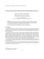
the separation process are presented in Figure 3. With
the input image shown in Figure 3a, the output images
and their histograms are also shown in Figure 3b,c,d,e
and Figure 3g,h,i,j, respectively. In the case of two subhistograms (n = 1), the output image lost some details in
the dark and light regions, so they are the main reasons of
unnatural visualization in the output. The degradation in

(2)

255

(i − μ2 (t))2 ωp(i)
2 (t)

i=t+1

where p(i) is the normalized histogram corresponding to
the probability density function of each gray value and
μi (t) are the class means which can be calculated as in the
following equations:
μ1 (t) =

t
i=0

μ2 (t) =

i×p(i)
ω1 (t)

.

255
i=t+1

(3)

i×p(i)
ω2 (t)

The weights ω1 (t) and ω2 (t) in Equations 1, 2, and 3 are
defined as
ω1 (t) =

t

p(i)
i=0

ω2 (t) =

.

255

p(i)
i=t+1

(4)

Figure 2 Mapping functions corresponding to cases of the Otsu
method separation.


Huynh-The et al. EURASIP Journal on Image and Video Processing 2014, 2014:44
/>
Page 4 of 17

Figure 3 The intermediate results of histogram equalization using the Otsu method for Lena image. (a) The original image. (b-e) The output
with n = 1, n = 2, n = 3, and n = 4, respectively. (f-j) The corresponding histograms of the images in (a-e).

Figure 3b can be explained through the mapping intensity
line (the red line in the Figure 2), in which the overenhancement occurs strongly in two ranges [0,100] and
[150,255]. These are the darker behavior at dark pixels
and the brighter behavior at bright pixels. In practice,
the larger the number of sub-histograms, the better the
images. However, the mapping functions became similar
to the uniform line f (k) = k in Figure 2, and the mean
of the output image brightness is close to the mean of the
input image brightness if the number of times in the separation is too large. The comparison of the proposed separation mechanism with the others such as BBHE, DSIHE,
MMBEBHE, and RSWHE is also represented in Table 1
as proof.
In this research, four sub-histograms are generated with
two times in separation process for avoiding the complex
computation and preserving the overall brightness. Let

us denote t1 , t2 , and t3 as the gray levels corresponding

to the separating points. There are four sub-histogram
ranges here as follows: [0, t1 ], [t1 + 1, t2 ], [t2 + 1, t3 ], and
[t3 + 1, L − 1]. Figure 4 shows the histogram sample
which is separated into four segments, called DR1, DR2,
DR3, and DR4 with lengths of (t1 + 1), (t2 − t1 ), (t3 − t2 ),
and (L − 1 − t3 ), respectively. Although the total length
of these sub-histograms is still L with L = 28 gray levels, there is a problem after separation when the authors
experienced many images: the performance of enhancement when the lengths of any sub-histograms are too
small.
Applying the histogram equalization algorithm for small
sub-histograms does not assure an effective enhancement
in the output due to a little bit of alteration. So these
sub-histograms could be resized by the controllable scale
factor and the fixed range to increase their lengths and
conserve the total gray level. The length of the fixed range,
called FR, depends on the number of sub-histograms that
are generated: FR = 2Ln = 64 for n = 2 with a total of
length L = 256. The lengths of resized dynamic ranges,

Table 1 Average of the means of 40 testing image
brightness (denoted as AMB)
Method

AMB
(50 images)

Original

120.98

BBHE [2]

133.27

DSIHE [3]

132.96

MMBEBHE [4]

123.97

RSWHE [12]

123.17

Proposed (2 sub-histograms)

135.05

Proposed (4 sub-histograms)

127.66

Proposed (8 sub-histograms)

123.77

Proposed (16 sub-histograms)

122.39

Figure 4 Example of the dynamic range separation using the
Otsu method with n = 2.


Huynh-The et al. EURASIP Journal on Image and Video Processing 2014, 2014:44
/>
denoted as RDR, of new sub-histograms are defined in the
following equation [8]:
RDRi = FR + α (DRi − FR)

i−1

RDRi

(6)

RDRi − 1.

(7)

k=1
i

maxi =
k=1

In Equation 5, the scale factor needs to be chosen carefully. When α = 1, the ranges of these sub-histograms
are invariable. The smaller the scale factor, the slighter
the effect of the Otsu method in separating the histogram. For α = 0, the total histogram was segmented
homogeneously, that is, the range of each partition is
constant and set at 64 as the fixed range. Figure 6 presented the output images and their histograms in the
cases that the scale factor was modified. Through intermediate results, it can be seen that the histogram in the
case of α = 0.9 looks similar to the one in the case of
non-resizing.
Contrast enhancement: histogram equalization for each
sub-histogram independently

Applying the HE approach for each sub-histogram independently is the next step in the BPWDRHE method.
With the gray-level k belonging to the ith new subhistogram (k ∈ [mini , maxi ]), the mapping function for
the current gray level as the input is given in the following
formula:

DR1
FR
RDR1

DR3
FR
RDR3

fhe (x) =

(5)

where α is the scale factor that has a value between 0
and 1. It is noted that the proposed separation in the

previous step is invalid when decreasing α to zero. The
examples of an original DR and new RDR after applying
a scale factor are shown in Figure 5. Let the range of the
new sub-histogram be [0, RDRi − 1] for the first one, and
[mini , maxi ] for ith one (with i > 1). Calculate the range of
the ith new sub-histogram through the equations below:
mini =

Page 5 of 17

DR2
FR
RDR2

DR4
FR
RDR4

Figure 5 Resizing the dynamic range with a scale factor α = 0.85
and number of times in separation n = 2.

⎧
⎪
⎪
⎪
⎨

x

(RDRi − 1)

k=0

⎪
⎪
⎪
⎩ (mini −1) + RDRi

nk
N1 ;
x
k=mini

(i = 1)
(8)
nk
Ni ; (i

> 1)

where nk is the number of pixels of gray-level k, and Ni
is the total pixels contained in the ith sub-histogram such
that N1 denotes the first sub-histogram.
Post-process: smooth the histogram and normalize the
brightness

The weakness of HE-based methods is that the HE histogram distribution is very scattered, that is, the distance between two non-zero pixel bins is large. It can
be explained by a few non-zero bins distributed on the
huge range. Because of the over-enhancement since this
behavior, the output images easily get visual artifacts. In

order to deal with this problem, the modified histogram
can be altered to be closer to the uniform distributed histogram, denoted as u. Using the algorithm for histogram
smoothing as suggested in [12], the mapping function is
defined as
fs (x) =

fhe + λu
(1 + λ) I + 2γ DT D

(9)

where λ is the uniform parameter and γ is the smoothing parameter, and the difference matrix D with a size of
length 255 × 256 is bi-diagonal:
⎡
⎤
−1 1 0 .. 0 0 0
D = ⎣ : : : .. : : : ⎦ .
(10)
0 0 0 .. 0 −1 1
The denominator in Equation 9, (1 + λ) I + 2γ DT D, in
fact corresponding to the term operates as the averaged
histogram function to make the histogram smoother. The
above term can be expressed explicitly and clearly as in the
matrix below:
⎡
⎤
2γ + (1 + λ)
−2γ
0
0 ···

⎢
−2γ
4γ + (1 + λ)
−2γ
0 ···⎥
⎢
⎥
.
⎢
0
−2γ
4γ + (1 + λ) −2γ · · · ⎥
⎣
⎦
..
..
..
.. . .
.
.
.
.
.
(11)
Let us examine Equation 9; when λ and γ are zero, the
smoothed histogram is equal to the HE histogram, that
is, there is no smoothing effect. In the case γ = 0, the
smoothed histogram becomes more similar to the uniform histogram when λ increases. If the uniform parameter is set at a constant value, the overall contrast of image
is reduced with the increment of γ . Figure 7a shows the
mapping function for smoothing HE with various uniform parameter λ while holding the smoothing parameter

Huynh-The et al. EURASIP Journal on Image and Video Processing 2014, 2014:44
/>
Page 6 of 17

Figure 6 The intermediate results of resizing for four sub-histograms. (a) The original image. (b-e) The output without resizing and resizing
with α = 0.1, α = 0.5, and α = 0.9, respectively. (f-j) The corresponding histograms of images in (a-e).

γ at zero. It is easy to realize that the mapping function
is close to the uniform distribution under increasing λ.
With λ ≥ 10, the line of mapping function is similar to
the that of the uniform. The histogram equalization hardly
has any influences in improving contrast if the uniform
parameter is too large. The effect of smoothing parameter in Equation 9 is shown in Figure 7b when the mapping
functions with λ ≥ 1 and modified smoothing parameter
γ were considered. In this case, the larger the smoothing
parameter γ , the softer the mapping function line. However, it is noted that the drawback of increasing γ is the
degrading overall contrast of the output image. Because of
the above reasons, choosing the unsuitable value of these
parameters can be a cause of degradation of image visualization. From the summarization shown in Figure 7c, the
case of λ = 1 and γ = 10 seems to be the best choice for
the smoothing step.
Finally, in order to minimize the difference between the
mean brightness of the output image and the original

(a)

image, the modified histogram is normalized by the
equation below [7]:

fn (x) =

B
fs (x)
Bs

(12)

where B and Bs are the mean brightness of the original
and modified image after using the smoothing algorithm,
respectively. The output image not only preserved the
overall brightness but also obtained the comfortable visualization by applying the mapping function as given in
Equation 12.

Results and discussions
For simulation, the authors compared the BPWDRHE
with the others which are the Global HE [1], BBHE [2],
DSIHE [3], MMBEBHE [4], WTHE [9], BPDHE [7],
RSWHE [10], and AGCWD [13] on various images. In
practice, 40 gray images [17] and 10 color images [18] of

(b)

(c)

λ

γ

λ

γ

λ

γ

λ

γ

λ

γ

λ

γ

λ

γ

λ
λ

γ

λ
λ

γ

λ
λ

γ
γ

λ

γ

γ

γ

Figure 7 Mapping function of smoothed HE image with various uniform λ and smoothing γ parameters. (a) γ = 0. (b) λ = 1. (c) The
summarization.


Huynh-The et al. EURASIP Journal on Image and Video Processing 2014, 2014:44
/>
the Kodak database set are utilized for quantitative measurement. Besides that, some random images are chosen
for representation and discussion. For more details, the
parameters and factors have been set in the proposed separation stage as follows: n = 2 corresponding to four
segments generated from the input histogram and α =
0.85 for resizing the lengths of sub-histograms. Moreover, with parameters in the post-process, the authors use
λ = 1 and γ = 10 to achieve efficiency in reducing negative effects from the over-enhancement and visual artifact
behavior. These parameters have been chosen through

the intermediate simulation, in which the experimental
results are represented in Figures 2 and 3 and Table 1
(for explanation of n), Figure 6 (for description of α), and
Figure 7 (for clarification of λ and γ ). It is important to
note that determined values for these parameters cannot be optimal for all images because the assessment for
image quality depends on various aspects. In this paper,
the authors try to estimate their values based on the observation of their specification. The influence of parameter
n is measured by the average mean brightness (AMB) as
shown in Table 1; meanwhile, the remaining parameters
are proposed to overcome unexpected events from the
histogram equalization scheme under visualization. However, the influence assessment of these parameters on the
overall performance of the output images is necessary to
be employed in the next simulation.
Assessment of the performance in contrast enhancement is never an easy mission. Although it is desirable
to have an objective assessment approach to compare
contrast enhancement techniques, unfortunately, there is
no accepted objective criterion in the literature to provide meaningful results for every image. However, there
are also some common quantitative measurements and
subjective assessments for the estimation. In this research,
the authors utilized the absolute mean brightness error
(AMBE) [5], the discrete entropy (DE) [12], and the measure of enhancement (EME) [19] as the quantitative measurements. It is important to notice that the contrast
enhancement for color images is quantified by applying
these measurements on only its luminance channel. For
the input image X and the output image Y, the AMBE is
defined in the following function as
AMBE = |E(X) − E(Y )|

(13)

where E(X) and E(Y ) are the mean brightness of the

images X and Y, respectively. The lower the value of the
AMBE, the better the preservation in brightness. The DE
of an image is described in the following function as
255

DE(X) = −

p (xi ) log p (xi )
i=0

(14)

Page 7 of 17

where p (xi ) is the probability of pixel intensity xi , which is
estimated from the normalized histogram. A higher value
of DE indicates that the image has richer details. In order
to calculate the EME, let us divide the image into k1 k2
non-overlapping sub-blocks Xi,j of size w1 × w2 , in this
paper; its size is chosen as 8 × 8 for assessment. The
parameter EME is computed in the following equation as
EME(X) =

1
k1 k2

k1

k2

20 ln
i=1 j=1

max Xi, j
min Xi, j

(15)

where max Xi, j and min Xi, j are the maximum and
minimum gray levels, respectively, in block Xi, j . Highcontrast sub-blocks give a high EME value, whereas for
homogeneous sub-blocks, the EME value should be close
to zero. It is worth to note that the EME is highly sensitive
to noise. However, for the contrast enhancement application, this value is expected to be EME(Y ) > EME(X).
In the next step, an evaluation of the proposed method
includes three simulations. Firstly, the authors assess the
influence of some parameters in the separation and postprocess stage on the overall performance with the quantitative and quality results. Then, the proposed method
is compared to the others with subjective assessment
for both gray-scale and color images. Finally, the comparison of the objective assessment based on the above
quantitative measurements is presented in detail.
Parameter assessment

To evaluate the influence of parameters like n, α, λ, and
γ , the authors decide to pick out a color sample from the
data to investigate. The visual results as the outputs are
presented in the Figures 8 and 9, while the quantitative
results are shown in Table 2. The information about the
values of these parameters corresponding to each image
can be referred through Table 2. Compared to the original image as shown in Figure 8a, the effect of parameter n
is recognized through Figure 8b,c,d. Although the changing in value of AMBE is very small, the DE and EME
results show the evident influence. The trade-off between

DE and EME can be realized as follows: when increasing
the number of segments in separation, the local contrast
factor (EME) will be decreased, while the measurement
of image detail is made to be greater. This statement is
verified through the observation of the cropping version
in Figure 9b,c,d. The objects in Figure 9b have high contrast; however, the texture of the white object is hardly
recognized. Since this sample does not belong to special
cases (no small sub-histogram is generated from the Otsu
separation), the effect of the resizing step by α is insignificant in the visualization (Figure 8e,f and Figure 9e,f ) and
also in the objective assessment (Table 2). For the uniform
parameter λ, the changes in overall performance occur
at all of the quantitative measurements. The increasing


Huynh-The et al. EURASIP Journal on Image and Video Processing 2014, 2014:44
/>
Page 8 of 17

Figure 8 The influence of parameters on the visual results at the outputs. (a) The original image. (b-j) The outputs corresponding to cases of
changing parameters (refer to Table 2 for more information).

value of λ will generate the output which looks similar
to the input (the values of DE and EME reach the original value). Finally, like the case of α, the impact of the
smoothing parameter γ is not enough to be detected, at
least for the visualization result, while it can be only recognized through the AMBE, DE, and EME with a little
bit of changing in value. With the proposed values for
these parameters (as in Figures 8c and 9c), the authors
want to achieve the balance of performance between the
visualization and quantitative results, in which it can be
seen that the values of AMBE, DE, and EME are homogeneously improved to get the stability for all images. That

means the overall contrast of the input image is enhanced
with the minimization of changes in brightness and loss in
detail.

Figure 9 The small region is cropped from Figure 8 (a-j).

Subjective assessment
Gray image

Some contrast enhancement results for gray-scale images
are shown in Figures 10, 11, 12, 13, 14 and 15 with three
samples named the Toy, the Aircraft, and the Pentagon.
For each image, the cropped version of the small area
is also represented clearly for analysis in detail. In order
to get the evident illustration of enhancement, Figure 16
presented the mapping functions of tested methods for
gray-scale images.
For the Toy image shown in Figure 10, due to the
over-contrast enhancement occurring abnormally in the
Global HE, it is hard to identify the plastic balloons. Some
methods including the BBHE, DSIHE, MMBEBHE, and
WTHE also provide similar contrast images; however, the


Huynh-The et al. EURASIP Journal on Image and Video Processing 2014, 2014:44
/>
Table 2 Quantitative assessment of parameters on the
overall performance
Figures 8 and 9 n
(a)

(c)

α

λ

γ

The original image
2

0.85

1

10

AMBE

DE

EME

-

3.7277

7.5317

0.0288 3.6578 10.8647

(b)

1

0.85

1

10

0.0334 3.6770 15.3762

(d)

3

0.85

1

10

0.0380 3.7005

(e)

2

0.5

1

10

0.0048 3.6734 10.6417

(f)

2

1

1

10

0.0308 3.6470 10.9212

(g)

2

0.85

5

10

0.1201 3.6892

8.6789

(h)

2

0.85 10

10

0.0960 3.7042

8.1405

(i)

2

0.85

1

1

0.0167 3.6409 11.1318

(j)

2

0.85

1

100

0.0479 3.7049 10.1021

9.2426

background of the output images is degraded seriously
with the rough brightness. The photometric differences
between some regions in the background are significant
and unacceptable. Therefore, the brighter regions can be
confused with the balloon shadows. The undesired behavior occurs severely in the output of the WTHE method.
Therefore, many artifacts and unnatural visualization
areas occur unexpectedly. Although getting a better visual
quality result, the enhancement of the AGCWD method
is not powerful enough to distinguish the details on
the balloon to observe as shown obviously in Figure 11.
The weakness of this method is not ensuring the overall brightness. For the BPDHE, RSWHE, and BPWDRHE
approaches, the outputs are not distorted in the global
contrast; however, the brightness of the RSWHE image is

Page 9 of 17

darker in general. In order to understand the effect of each
approach, Figure 16a displays their mapping functions. In
the gray-value range [0,40], the behaviors of some methods, such as the Global HE, BBHE, DSIHE, MMBEBHE,

WTHE, and BPDHE, are similar and therefore it explained
for the dark areas on the balloons. In addition, the decay
of illumination on the background is clarified by the shape
of mapping lines in the range [190,255].
For both the Aircraft image and its cropped area
shown in Figures 12 and 13, it can be seen that some
approaches, such as the Global HE, BBHE, MMBEBHE,
and WTHE, enhanced the overall brightness excessively
and therefore the texture on the aircraft body cannot be
observed clearly. Although the DSIHE and BPDHE methods perform better than the above methods, they also
enhanced some unnecessary details on the background.
Observation of the contrast enhancement on the RSWHE
image is quite difficult due to the slight effect. For the
AGCWD method, the enhanced image looks brighter
without brightness preservation and so many bright-pixel
details have been removed, such as the take-off trail.
Meanwhile, the proposed approach enhances the contrast
at the moderate level enough to observe each component
of the aircraft body and the take-off trail clearly without
an alteration in the brightness. The shapes of mapping
function lines of some bad visualization schemes, such as
the Global HE, BBHE, and WTHE, are alike. The limitation of the value range in the WTHE technique can
be understood as the main reason for a low contrast in
the output. The behavior of the MMBEBHE line in the
range [60,150] is the cause of losing details on the aircraft body. Since the RSWHE line is close to the uniform

Figure 10 Comparison of enhancement methods with test image Toy. (a) Original. The enhanced image: (b) Global HE. (c) BBHE. (d) DSIHE.
(e) MMBEBHE. (f) WTHE. (g) BPDHE. (h) RSWHE. (i) AGCWD. (j) BPWDRHE.

Huynh-The et al. EURASIP Journal on Image and Video Processing 2014, 2014:44
/>
Page 10 of 17

Figure 11 The small region is cropped from Toy. (a) Original. The enhanced image: (b) Global HE. (c) BBHE. (d) DSIHE. (e) MMBEBHE. (f) WTHE.
(g) BPDHE. (h) RSWHE. (i) AGCWD. (j) BPWDRHE.

line, the output looks like the input in the contrast. For
the BPWDRHE method, the gray-value ranges [0,40] and
[200,250] corresponding to the bright and dark pixels are
improved fairly.
Some methods including the Global HE, BBHE,
MMBEBHE, and WTHE methods improved the contrast
of image excessively in the two-side extension way in the
Pentagon image: the bright pixels to be even brighter
and the dark pixels to be even darker. As a result,

some dark and bright details can be damaged seriously.
The three methods such as the BPDHE, RSWHE, and
BPWDRHE still maintain the general brilliance. However, some regions in the enhanced image of the BPDHE
method are dimmed unexpectedly with medium brightness pixels, while an enhancement of the RSWHE method
is not strong enough to recognize the modification in
the contrast. In practice, these observations are displayed
in detail in Figure 15. Except for the fan-shaped object

Figure 12 Comparison of enhancement methods with test image Aircraft. (a) Original. The enhanced image: (b) Global HE. (c) BBHE. (d)
DSIHE. (e) MMBEBHE. (f) WTHE. (g) BPDHE. (h) RSWHE. (i) AGCWD. (j) BPWDRHE.


Huynh-The et al. EURASIP Journal on Image and Video Processing 2014, 2014:44

/>
Page 11 of 17

Figure 13 The small region is cropped from Aircraft. (a) Original. The enhanced image: (b) Global HE. (c) BBHE. (d) DSIHE. (e) MMBEBHE. (f)
WTHE. (g) BPDHE. (h) RSWHE. (i) AGCWD. (j) BPWDRHE.

in the square detected by the very dim thin boundary in Figure 15b,c,d,e,f, the BPDHE image also gets the
same behavior with medium gray levels. Only with the
RSWHE and BPWDRHE methods can the object be identified easily due to its high contrast. The shape of the
mapping function line in Figure 16c of the AGCWD
approach in the range [125,255] explained for the brightened image. Due to getting the same result in the enhancement, the lines of the Global HE, BBHE, and MMBEBHE

methods are similar to each other. The gray-level limitation in the WTHE and BPDHE produces low-contrast
images in the output when the maximum gray value is
200 and 206 instead of 255 as normality. After all, the
behavior of the mapping function line of the proposed
method at the ranges [0,73] and [190,255] for contrast
improvement and [105,170] for brightness preservation produced the pleasing visualization in the output
image.

Figure 14 Comparison of enhancement methods with test image Pentagon. (a) Original. The enhanced image: (b) Global HE. (c) BBHE. (d)
DSIHE. (e) MMBEBHE. (f) WTHE. (g) BPDHE. (h) RSWHE. (i) AGCWD. (j) BPWDRHE.


Huynh-The et al. EURASIP Journal on Image and Video Processing 2014, 2014:44
/>
Page 12 of 17

Figure 15 The small region is cropped from Pentagon. (a) Original. The enhanced image: (b) Global HE. (c) BBHE. (d) DSIHE. (e) MMBEBHE.
(f) WTHE. (g) BPDHE. (h) RSWHE. (i) AGCWD. (j) BPWDRHE.

Color image

Contrast enhancement can be easily extended to the color
images. The most obvious way to extend the color images
is to apply these methods to the luminance component.
However, some enhancement approaches for color images
utilized the HSV (hue, saturation, value) [14] color model
to improve the contrast. To consider the performance
of the tested method for color images, the simulation
was implemented for ten color images from the Kodak
standard image library. At first, the sample color image
Hats is shown in Figure 17 and the cropped version in
Figure 18. In the results of the Global HE, BBHE, DSIHE,
and WTHE methods, the hues of the output images are
changed seriously. These studies not only darkened some
areas of the wood plank and the hat shadows but also

(a)

brightened some regions of the cloud and the top of the
yellow hat. Therefore, many features in these regions are
lost. The degradations of the MMBEBHE, WTHE, and
BPDHE approaches are not as severe as the result of
the above methods. To be better, the AGCWD method
produced the brighter image both in overall and detail;
however, recognition of the bright-pixel details on the top
of the yellow hat is an impossible task due to its bad contrast. Only with the proposed method and the RSWHE are
the details enhanced expectantly with no hue distortion,
for instance, the texture of the wood plank looks clear.

Based on the mapping function as shown in Figure 19a,
it is not difficult to realize that the Global HE, BBHE,
DSIHE, and WTHE methods enhanced over-contrast for
the bright pixels corresponding to the pixels in the range

(b)

Figure 16 Mapping functions of three gray-scale images. (a) The Toy. (b) The Aircraft. (c) The Pentagon.

(c)


Huynh-The et al. EURASIP Journal on Image and Video Processing 2014, 2014:44
/>
Page 13 of 17

Figure 17 Comparison of enhancement methods with test image Hats. (a) Original. The enhanced image: (b) Global HE. (c) BBHE. (d) DSIHE.
(e) MMBEBHE. (f) WTHE. (g) BPDHE. (h) RSWHE. (i) AGCWD. (j) BPWDRHE.

[150,255] and the dark pixels corresponding to the pixels
in the range [0,50]. The distortion in the hue component
of the cloud and the wood plank can be explained by
this behavior. For this sample, only the overall contrast
of the AGCWD method is limited. The output images
of the RSWHE and BPWDRHE approaches look natural
with the enhancement process for both dark-pixel range
[0,75] and bright-pixel range [175,255]. Nevertheless, the
modification on the output image after improving the
contrast in the RSWHE case is not obvious.
The Wall image, the next color sample, is shown in

Figures 20 and 21. The results of the Global HE, BBHE,
DSIHE, MMBEBHE, and WTHE have similar contrast
enhancement with cold overall hue, while BPDHE has a

better visual result. The characteristic of the AGCWD
is that it usually produces the output images which are
brighter than the original. Therefore, some bright-pixel
details having a low-contrast will be lost or realized with
difficulty. In Figure 21, the object behind the glass window
in the Global HE, BBHE, DSIHE, and WTHE methods
is brightened so much that it is hardly observed. Except
for the RSWHE and BPWDRHE, the remaining methods
get the same drawback in the slight level. Considering
the chroma of the door, it can be seen that the enhancement of the RDWHE mechanism is very slight. For the
BPWDRHE method, the output image achieves adequate
contrast in both the overall and detail. The input to output gray-level functions of the tested methods can be

Figure 18 Comparison of enhancement methods with test image Hats (cropped from Figure 17). (a) Original. The enhanced image:
(b) Global HE. (c) BBHE. (d) DSIHE. (e) MMBEBHE. (f) WTHE. (g) BPDHE. (h) RSWHE. (i) AGCWD. (j) BPWDRHE.


Huynh-The et al. EURASIP Journal on Image and Video Processing 2014, 2014:44
/>
(a)

Page 14 of 17

(b)

Figure 19 Mapping functions of two color images. (a). The Hats (b). The Wall.

carefully considered in Figure 19b. The common shortcoming of the Global HE, BBHE, MMBEBHE, DSIHE,
and WTHE is the production of the over-contrast images.
The output images of these methods lose the bright and
dark pixel parts. Based on the mapping function lines in
Figure 19b, the pixels belonging to the range [0,50] will be
darkened, while the pixels in the range [175,255] become
lighter for the above methods. Therefore, details of the
object behind the glass window are removed unexpectedly. Like the previous test images, the AGCWD has a
tendency to produce a brighter image for the gray level
larger than 50, while the overall contrast has not been preserved. The BPDHE method is similar to the AGCWD in
the range [150,255]; however, it gets the same behavior of
the Global HE for the over-contrast enhancement. Only
two methods, the RSWHE and BPWDRHE, get the good
enhancement when only improving the luminance in the
sensible level. Nevertheless, the input to output function
of the proposed method is smoother than that of the
RSWHE.

Objective assessment

Results of the AMBE, DE, and EME measurement of 50
sample images are listed in Tables 3, 4 and 5, respectively.
In Table 3, the average value of AMBEs is shown beside the
results of sample images which were presented in the subjective assessment. A comparison of AMBE values shows
that the proposed method and the BPDHE outperform
others used in the simulation when they achieve good
brightness preservation with the smallest values by the
brightness normalization after equalizing the histogram.
Due to focusing on brightness improvement for dimmed

images without brightness preservation, the AGCWD
method has the greatest value of AMBE when this method
made inputs to be brighter in most of the output images.
Without any solutions to limit the modification in the
overall brightness, the remaining methods produce unexpected images which are different from the original in
the global brightness. Based on the results of the Aircraft
sample in Figure 12, it is not difficult to predict the brightness error when AMBE values of outputs of the Global

Figure 20 Comparison of enhancement methods with test image Wall. (a) Original. The enhanced image: (b) Global HE. (c) BBHE. (d) DSIHE.
(e) MMBEBHE. (f) WTHE. (g) BPDHE. (h) RSWHE. (i) AGCWD. (j) BPWDRHE.


Huynh-The et al. EURASIP Journal on Image and Video Processing 2014, 2014:44
/>
Page 15 of 17

Figure 21 Comparison of enhancement methods with test image Wall (cropped from Figure 20). (a) Original. The enhanced image:
(b) Global HE. (c) BBHE. (d) DSIHE. (e) MMBEBHE. (f) WTHE. (g) BPDHE. (h) RSWHE. (i) AGCWD. (j) BPWDRHE.

HE, DSIHE, WTHE, and AGCWD are so much higher
than others. These methods generate the outputs to be
either so much darker or brighter. The BBHE and DSIHE
have the same idea in the histogram separation; thus, their
AMBE values look similar together, except for some cases
of special histograms. Meanwhile, the MMBEBHE gets
the better result because its algorithm not only improves
the contrast like BBHE but also minimizes the total error
of brightness changes.
With the second measurement, the DE of the original image will be seen as the standard to be compared
with the DE of enhanced images. The important thing to

note is that the DE values of modified images are always
equal or less than the original. This means that it is difficult to retain the detail of the output like the detail of
the input. The behavior of losing detail occurs in most

of the enhancement methods because the mapping function is nonlinear, that is, it usually has one output value
for many input values. This behavior is absolutely considered through mapping function graphs as in Figures 16
and 19. The other way to explain based on histograms is
that many original histogram bins grouped into one bin
after enhancement can be the reason of the decrement in
the DE values for over-enhanced images. It is not difficult
to understand why the DE parameter of output images of
these approaches is slightly reduced. Through Table 4, the
performance of the proposed method and the RSWHE are
quite similar in the average value of DE when both of them
with high discrete entropy are better than the other methods. The Global HE gives the worst results in most of the
samples with the least value of average as the loss of data
of over 15%, while the remaining methods basically keep

Table 3 Absolute mean brightness error (AMBE) and average of AMBEs (AAMBE)
AMBE
Method

Toy

Aircraft

Pentagon

Global HE [1]

29.38

47.82

BBHE [2]

5.48

1.46

DSIHE [3]

1.27

MMBEBHE [4]

3.16

WTHE [9]
BPDHE [7]

AAMBE
Hats

Wall

(50 images)

11.04

7.81

10.19

30.49

6.89

23.77

17.19

12.29

15.42

28.65

0.03

10.19

11.98

6.51

1.37

1.25

1.00

2.99

27.13

55.61

12.36

22.25

23.62

29.62

0.15

0.05

0.02

0.02

0.007

0.26

RSWHE [10]

7.70

3.48

0.80

0.76

0.45

2.19

AGCWD [13]

26.14

58.45

35.46

33.52

38.33

36.75

BPWDRHE

0.08

0.01

0.09

0.02

0.07

0.05


Huynh-The et al. EURASIP Journal on Image and Video Processing 2014, 2014:44
/>
Page 16 of 17

Table 4 Discrete entropy (DE) and average of DEs (ADE)
DE
Method

Toy

ADE

Aircraft

Pentagon

Hats

Wall

(50 images)

Original

4.19

2.78

4.66

4.79

4.83

4.52

Global HE [1]

3.48

2.60

4.01

4.66

4.75

3.84

BBHE [2]

4.09

2.72

4.61

4.1

4.11

4.42

DSIHE [3]

4.03

2.74

4.57

4.67

4.75

4.40

MMBEBHE [4]

4.07

2.71

4.59

4.65

4.74

4.41

WTHE [9]

3.35

2.74

4.64

4.68

4.70

4.27

BPDHE [7]

4.07

2.75

4.47

4.60

4.58

4.32

RSWHE [10]

4.19

2.78

4.66

4.79

4.83

4.51

AGCWD [13]

3.61

2.78

4.62

4.74

4.79

4.30

BPWDRHE

4.15

2.77

4.64

4.77

4.81

4.48

image content at the moderate level with the largest losing
grade of 6%.
The comparison of EME values in Table 5 shows that
the Global HE, BBHE, DSIHE, MMBEBHE, and WTHE
methods usually get higher EME values than the remaining methods. Since the EME criterion measures a form
of contrast, it is no surprise that these methods give the
highest values even though they hardly ever produced

the most visually pleasing images. Although the enhancement grade is identified through this value with the output
value greater than the value of the original image, the high
results of the above methods can be the main reason for
the degradation of quality. As results for the Toy sample, some methods such as the Global HE, BBHE, DSIHE,
MMBEBHE, and WTHE achieve the high value of EME
corresponding to the high contrast; however, their outputs
are seriously damaged unexpectedly in the quality. For the
AGCWD method, increasing the brightness overall can
be the cause of depressing the local contrast corresponding to the EME value, especially with the Aircraft sample.
Meanwhile, the EME values achieved from the proposed

method are enough to realize the difference of contrast
between inputs and outputs without visual artifacts.
In summary, it is important to note that the quality of
an enhanced image depends on many criteria. Besides
increasing the contrast in the adequate grade to avoid the
occurrence of artifact unexpectedly, the efficient method
needs to preserve not only the overall brightness but also
the detail in the output. Based on the experimental results,
the proposed method satisfied these criteria at least in this
evaluation with 50 test images; however, the trade-off here
is the computation fee, that is, the algorithm will need
more time for enhancing the steps.

Conclusion
In this work, the authors proposed and experimented on
the new contrast enhancement method for both grayscale and color image, called BPWDRHE. The BPWDRHE
method enhanced the contrast with preservation of the
overall brightness to generate the natural looking images.
Unlike some previous techniques, the proposed method

reduced the appearance of visual artifacts in the outputs.

Table 5 Measure of enhancement (EME) and average of EMEs (AEME)
EME

AEME

Method

Toy

Aircraft

Pentagon

Hats

Wall

(50 images)

Original

4.81

3.14

8.59

5.42

14.65

14.34

Global HE [1]

13.94

25.64

40.57

15.64

39.87

28.86

BBHE [2]

10.99

18.99

36.44

15.85

42.56

26.04

DSIHE [3]

9.40

8.09

21.62

15.91

39.86

23.88

MMBEBHE [4]

11.06

8.72

23.96

14.28

38.07

24.27

WTHE [9]

10.34

15.39

32.5

12.89

34.92

22.44

BPDHE [7]

7.18

5.68

14.71

12.76

19.55

21.09

RSWHE [10]

6.60

3.37

10.16

7.03

16.65

15.12

AGCWD [13]

4.61

1.98

8.56

5.55

14.44

14.19

BPWDRHE

6.29

4.85

12.28

7.62

20.87

15.62


Huynh-The et al. EURASIP Journal on Image and Video Processing 2014, 2014:44
/>
The novelty of proposed contrast enhancement is that
the sum of weighted within-class variance was utilized
to determine the break points for histogram separation
based on the minimization of the total squared error of
each sub-histogram corresponding to the equalizationbased brightness shift. After applying the HE technique
for these sub-histograms, the output image histogram will
be smoothed and normalized to obtain the good visualization as the post-processes. Moreover, the BPWDRHE
was estimated for gray-scale and color images and then
compared to the others in various aspects with some common quantitative assessments, such as the absolute mean
brightness error, the discrete entropy, and the measure of
enhancement.
Competing interests
The authors declare that they have no competing interests.

Page 17 of 17

13. S-C Huang, F-C Cheng, Y-S Chiu, Efficient contrast enhancement using
adaptive gamma correction with weighting distribution. IEEE Trans.
Image Process. 22(3), 1032–1041 (2013)
14. Z Zhou, N Sang, X Hu, Global brightness and local contrast adaptive
enhancement for low illumination color image. Optik - Int. J. Light
Electron Opt. 125(6), 1795–1799 (2014)
15. A Draa, A Bouaziz, An artificial bee colony algorithm for image contrast
enhancement. Swarm Evol. Comput. 16, 69–84 (2014)
16. M Abdullah-Al-Wadud, MH Kabir, MAA Dewan, O Chae, A dynamic
histogram equalization for image contrast enhancement. IEEE Trans.
Consum. Electron. 53(2), 593–600 (2007)
17. The USC-SIPI Image Database. Accessed 20
Jan 2013
18. Kodak Lossless True Color Image Suite. />Accessed 5 August 2013
19. SS Agaian, B Silver, KA Panetta, Transform coefficient histogram-based
image enhancement algorithms using contrast entropy. IEEE Trans.
Image Process. 16(3), 741–758 (2007)
doi:10.1186/1687-5281-2014-44
Cite this article as: Huynh-The et al.: Using weighted dynamic range for
histogram equalization to improve the image contrast. EURASIP Journal on
Image and Video Processing 2014 2014:44.

Acknowledgements
This research was funded by the MSIP (Ministry of Science, ICT & Future
Planning), Korea in the ICT R&D Program 2013.
Author details
1 Department of Computer Engineering, Kyung Hee University, 1732
Deokyoungdae-ro, Giheng-gu, Youngin-si, Seoul, Gyeonggi-do 446-701, Korea.
2 Department of Electrics and Electronics Engineering, Ho Chi Minh City
University of Technology, 268, Ly Thuong Kiet, District 10, Ho Chi Minh 70000,

Vietnam. 3 Department of Multimedia Science, Sookmyung Women University,
Cheongpa-ro 47-gil 100, Youngsan-gu, Seoul 140-742, Korea.
Received: 27 March 2014 Accepted: 29 August 2014
Published: 13 September 2014
References
1. RC Gonzalez, RE Woods, Digital Image Processing, 3rd Edition. (Prentice
Hall, New Jersey, 2007)
2. Y-T Kim, Contrast enhancement using brightness preserving bi-histogram
equalization. IEEE Trans. Consum. Electron. 43(1), 1–8 (1997)
3. Y Wang, Q Chen, B Zhang, Image enhancement based on equal area
dualistic sub-image histogram equalization method. IEEE Trans. Consum.
Electron. 45(1), 68–75 (1999)
4. S-D Chen, AR Ramli, Minimum mean brightness error bi-histogram
equalization in contrast enhancement. IEEE Trans. Consum. Electron.
49(4), 1310–1319 (2003)
5. S-D Chen, AR Ramli, Contrast enhancement using recursive
mean-separate histogram equalization for scalable brightness
preservation. IEEE Trans. Consum. Electron. 49(4), 1301–1309 (2003)
6. KS Sim, CP Tso, YY Tan, Recursive sub-image histogram equalization
applied to gray scale images. Pattern Recogn. Lett. 28(10), 15 (2007)
7. H Ibrahim, NSP Kong, Brightness preserving dynamic histogram
equalization for image contrast enhancement. IEEE Trans. Consum.
Electron. 53(4), 1752–1758 (2007)
8. G-H Park, H-H Cho, M-R Choi, A contrast enhancement method using
dynamic range separate histogram equalization. IEEE Trans. Consum.
Electron. 54(4), 1981–1987 (2008)
9. Q Wang, RK Ward, Fast image/video contrast enhancement based on
weighted thresholded histogram equalization. IEEE Trans. Consum.
Electron. 53(2), 757–764 (2007)
10. M Kim, M Chung, Recursively separated and weighted histogram

equalization for brightness preservation and contrast enhancement.
IEEE Trans. Consum. Electron. 54(3), 1389–1397 (2008)
11. N Sengee, H Choi, Brightness preserving weight clustering histogram
equalization. IEEE Trans. Consum. Electron. 54(3), 1329–1337 (2008)
12. T Arici, S Dikbas, Y Altunbasak, A histogram modification framework and
its application for image contrast enhancement. IEEE Trans. Image
Process. 18(9), 1921–1935 (2009)

Submit your manuscript to a
journal and benefit from:
7 Convenient online submission
7 Rigorous peer review
7 Immediate publication on acceptance
7 Open access: articles freely available online
7 High visibility within the field
7 Retaining the copyright to your article

Submit your next manuscript at 7 springeropen.com