Choice of location, growth and welfare with unequal pollution exposures
Bạn đang xem bản rút gọn của tài liệu. Xem và tải ngay bản đầy đủ của tài liệu tại đây (1.3 MB, 27 trang )
This article was downloaded by: [Umeå University Library]
On: 03 April 2015, At: 16:24
Publisher: Taylor & Francis
Informa Ltd Registered in England and Wales Registered Number: 1072954
Registered office: Mortimer House, 37-41 Mortimer Street, London W1T 3JH, UK
Technological and Economic
Development of Economy
Publication details, including instructions for authors and
subscription information:
/>
Choice of location, growth and
welfare with unequal pollution
exposures
a
b
Hoang Khac Lich & Frédéric Tournemaine
a
University of Economics and Bussiness, Vietnam National
University, Hanoi, 144 Xuan Thuy, Cau Giay, Hanoi, Vietnam
b
School of Economics, University of the Thai Chamber of
Commerce, 126/1 Vibhavadee-Rangsit Road, Dindaeng,
Bangkok, 10400, Thailand
Published online: 28 Jan 2014.
To cite this article: Hoang Khac Lich & Frédéric Tournemaine (2013) Choice of location, growth
and welfare with unequal pollution exposures, Technological and Economic Development of
Economy, 19:sup1, S58-S82
To link to this article: />
PLEASE SCROLL DOWN FOR ARTICLE
Taylor & Francis makes every effort to ensure the accuracy of all the information (the
“Content”) contained in the publications on our platform. However, Taylor & Francis,
our agents, and our licensors make no representations or warranties whatsoever
as to the accuracy, completeness, or suitability for any purpose of the Content. Any
opinions and views expressed in this publication are the opinions and views of the
authors, and are not the views of or endorsed by Taylor & Francis. The accuracy
of the Content should not be relied upon and should be independently verified
with primary sources of information. Taylor and Francis shall not be liable for any
losses, actions, claims, proceedings, demands, costs, expenses, damages, and other
liabilities whatsoever or howsoever caused arising directly or indirectly in connection
with, in relation to or arising out of the use of the Content.
This article may be used for research, teaching, and private study purposes. Any
substantial or systematic reproduction, redistribution, reselling, loan, sub-licensing,
systematic supply, or distribution in any form to anyone is expressly forbidden. Terms
Downloaded by [Umeå University Library] at 16:24 03 April 2015
& Conditions of access and use can be found at />terms-and-conditions
Technological and economic development OF ECONOMY
ISSN 2029-4913 print/ISSN 2029-4921 online
2013 Volume 19(Supplement 1): S58–S82
doi:10.3846/20294913.2013.869668
CHOICE OF LOCATION, GROWTH AND WELFARE
WITH UNEQUAL POLLUTION EXPOSURES
Downloaded by [Umeå University Library] at 16:24 03 April 2015
Hoang Khac LICHa, Frédéric TOURNEMAINEb
University of Economics and Bussiness, Vietnam National University, Hanoi,
144 Xuan Thuy, Cau Giay, Hanoi, Vietnam
b
School of Economics, University of the Thai Chamber of Commerce,
126/1 Vibhavadee-Rangsit Road, Dindaeng, Bangkok, 10400, Thailand
a
Received 26 December 2011; accepted 26 May 2012
Abstract. We develop an endogenous growth model with human capital accumulation in which
firms are polluting and heterogeneous individuals must decide, among other things, where to
live. The main idea is that pollution is unequally spread across geographical locations, inducing
a trade-off for individuals between environmental quality and leisure. In such economy, we show
that a better environmental quality and/or a greater degree of inequality lead individuals to favour
cleaner locations which, in turn, boosts long-term growth. Welfare-wise, we find that, in general,
individuals prefer a greater level of consumption and leisure but lower growth and environmental
quality than those which are possible to achieve. Moreover, we show that the sign of the impact of
inequality on environmental quality is likely to be negative.
Keywords: location choice, growth, inequality, welfare, environmental quality.
Reference to this paper should be made as follows: Lich, H. K.; Tournemaine, F. 2013. Choice of
location, growth and welfare with unequal pollution exposures, Technological and Economic Development of Economy 19(Supplement 1): S58–S82.
JEL Classification: O31, O41, Q28.
Introduction
Beside the decisions on the amount of consumption and leisure they purchase, another
key variable that enters in individuals’ optimization problem is the geographical location
for housing. This is an important decision variable because it affects welfare both directly
and indirectly in several ways. For instance, housing location, via the distance to travel to
Corresponding author Frédéric Tournemaine
E-mail: ,
Copyright © 2013 Vilnius Gediminas Technical University (VGTU) Press
/>
Downloaded by [Umeå University Library] at 16:24 03 April 2015
Technological and Economic Development of Economy, 2013, 19(Supplement 1): S58–S82
S59
the working place and the time it requires for its purpose, determines the amount of leisure
individuals must give up in addition to their working time. The distance between housing
location and working place also involves monetary costs: Glaeser et al. (2008), for instance,
clearly establish that the cost of automobiles is a relevant factor explaining why poor people
often live in the vicinity of the place where they work, while richer individuals choose to live
further away. Last, but not least, as many epidemiological studies suggest, location choices
determine the pollution burden individuals face. For instance, as emphasized by O’Neill
et al. (2003), pollution exposure and vulnerability are unequally spread across individuals
and mainly depend on their geographical location. This analysis shows in particular that
poor individuals tend to live more often in most polluted areas, a feature corroborated by
several articles discussing the link between location of households, income and pollution
exposure (Michaels, Smith 1990; Kohlhase 1991; Kiel, McClain 1995; McCluskey, Rausser
2003; Kohlhuber et al. 2006; Levy 2009; Su et al. 2011): this literature shows indeed that
poorer individuals tend to live closer to their working place (often characterized by a higher
burden of pollution emissions) because it allows them to reduce their cost of commuting to
work and housing expenses1.
In this context and in light of the well recognized and documented effects of pollution
on individuals’ health, we can infer that such pattern in individuals’ geographical location
can have important economy-wide consequences, specifically for the determination and interplay of economic variables such as the level of long-term growth and individuals’ welfare.
As argued by Aloi and Tournemaine (2011, 2013) among others, pollution is a serious and
growing problem, particularly in rapidly expanding cities, causing a considerable threat to
human health. The problem is that poor health produces significant economic losses not
only because it affects individuals’ participation to the labour market, but also because it
affects individuals’ learning abilities. The reason is that health is an important component of
human capital which itself is a key engine of long-term growth (Lucas 1988). In other words,
capturing the above features in a simple theoretical framework and analyzing the location
choices of individuals together with environmental problems in an endogenous growth
model is a relevant issue.
In this paper, we explore the impact of inequality and environmental quality on individuals’ location choices and determine how it translates to long-term growth, welfare and
the relationship between the two. In comparison to existing literature, this article brings a
different theoretical perspective as it raises the issue of whether equity, growth and welfare
can be mutually compatible, in a context where pollution exposure is uneven and growth and
location choices are both endogenous. In the standard theoretical environmental literature,
1
It is important to mention that we will formalize the centre of economic activity as the place where polluting
activities (firms) are located. We should keep in mind, however, that the assertion that poorer households live
near the central business district is not always exact. Interested readers could for instance refer to Brueckner
et al. (1999) among others who have shown that the relative location of individuals depends on the cities’ spatial
pattern of amenities (a result which, as seen above, is confirmed empirically by Glaeser et al. 2008). The pattern
of location with respect to pollution, however, which is at the centre of our analysis, seems to be a more common
observation. Moreover, as we will see shortly, our simplifying formalization will allow us to capture the fact that,
as they become richer, individuals are willing to pay higher transportation costs and housing prices to benefit from
a better environmental quality.
Downloaded by [Umeå University Library] at 16:24 03 April 2015
S60
H. K. Lich, F. Tournemaine. Choice of location, growth and welfare with unequal pollution...
Gradus and Smulders (1993), van Ewijk and van Wijnbergen (1995) and Pautrel (2008, 2009),
among others, have demonstrated how the negative impact of pollution on learning abilities
of individuals can be transmitted to economic growth and shown that a better environmental
quality and a higher long-term level of growth are mutually compatible. However, in their
models, agents are assumed identical in all dimensions. Moreover, they did not take into
account either that pollution is unequally spread across geographical locations, nor the idea
that housing location is a decision variable.
In this paper, in contrast, we follow Aloi and Tournemaine (2013) as we develop an
endogenous growth model “a la Lucas (1988)” in which heterogeneous individuals must
decide not only their level of consumption and the amount of resources to invest in human
capital accumulation, but also the place to live (i.e. the distance to commute to work) and
their labour supply.
Following Blanchard (2004), heterogeneity across individuals stems from the marginal
disutility individuals obtain from non leisure activities, i.e. the time spent at work and that
used for commuting to work. The key idea of the model is to formalize a trade-off between
environmental quality which affects individuals’ learning abilities, and leisure. Specifically,
when individuals choose to live closer to the firm, they suffer greater health shortfalls and
accumulate less human capital due to the greater impact of pollution coming from production; but on the other hand, they obtain more leisure time as they have a shorter distance
to travel to work2. We then emphasize the role of environmental quality as a determinant of
individuals’ location choices, both serving as possible factors affecting their learning abilities,
and in turn the level of long-term growth and their welfare.
Close to our analysis, are also the works by Eriksson and Persson (2003) and Kempf and
Rossignol (2007) who develop models with heterogeneous individuals. Eriksson and Persson
also assume that pollution is unevenly spread across individuals. They study the effect of
heterogeneity in income and pollution, together with the society’s level of democratization,
on environmental policy choices and show that a more even income distribution and more
democracy lead to improvements in environmental quality. Kempf and Rossignol (2007)
use an AK model with a pollution externality. Their main result is to show that, in general,
poorer individuals favour less stringent environmental policies. However, they ignore that
pollution exposure and vulnerability disproportionally affect poorer individuals. However,
contrary to ours, their model does not analyze how reducing pollution influences growth
through the channel of human capital accumulation. This is an important difference since,
as emphasized before, the effects of pollution on health and learning abilities represent one
of the largest gains from environmental regulation.
Our main results can be summarized as follows. First, we show that a tighter environmental policy always increases individuals’ distance of commuting to work. The intuition
behind this result is simple. As environmental quality increases, individuals accumulate a
greater amount of human capital synonymous of a greater productivity. As a result, they
obtain a greater income and become more willing to reduce their amount of leisure to
2
We will see that leisure time increases because individuals reduce their labour supply when they live closer to the
firm, source of pollution. The reason is that, in choosing a location near the firm, where pollution is high, individuals
accumulate less human capital, i.e. they have a lower productivity.
Downloaded by [Umeå University Library] at 16:24 03 April 2015
Technological and Economic Development of Economy, 2013, 19(Supplement 1): S58–S82
S61
enjoy a better environmental quality. Second, in contrast with Gradus and Smulders (1993),
van Ewijk and van Wijnbergen (1995) and Pautrel (2008, 2009) who find a monotonic
relationship between growth and the policy level, we obtain an inverted-U relationship
implying the existence of a growth-maximizing policy level. The rationale behind our
result is similar to that described in Barro (1990) on the contribution of public services to
growth and welfare. In our set up, the environmental policy tool is similar to a fund raising
vehicle for abatement investments. Thereby, abatements play a comparable role to public
infrastructures, in that the growth-maximizing (abatement) policy reflects two aspects.
On the one hand, it reflects the contribution of abatements to the reduction of pollution
emissions, which improves the productivity of individuals through their human capital
accumulation process. On the other hand, it reflects a resource withdrawal effect, as more
resources devoted to abatements have a negative effect on individuals’ private investments
in the human capital sector.
From a welfare point of view, however, although the theory predicts an ambiguous outcome, the economic intuition and numerical calibration of the model show that, in general,
individuals are likely to favour an abatement policy level which is lower than the growth-maximizing one. In other words, the model predicts that, in the most plausible scenario, a greater
amount of funds allocated to abatement activities is not only environment and welfare
improving but also growth enhancing. Moreover, as we show that the welfare maximizing
abatement policy depends on the degree of heterogeneity across individuals (inequality), we
can give a simple explanation to the empirical observation according to which an increase in
inequality seems to be positively correlated with a reduction in environmental quality (Torras, Boyce 1998; Magnani 2000): formally, we show that a greater degree of inequality across
individuals can lead to a reduction of the welfare maximizing abatement policy, synonymous
of a greater level of consumption and leisure.
The remainder of the paper is structured as follows. We introduce the model in Section 1.
In Section 2, we characterize the equilibrium in which we analyze the abatement policy
implications on individuals’ location choices, growth and welfare. We finally provide the
conclusions of the analysis.
1. Model
The main building block of the model is taken from Aloi and Tournemaine (2013). Consider
a closed economy in continuous time populated by a mass 0,N of infinitely-lived individuals who live in a city represented by a segment of exogenous length, 0, α max . Each
individual is endowed with hi ,0 = 1 unit of human capital at date zero and must decide the
amount of resources to allocate between private consumption and human capital accumulation, the amount of time to work and also the place to live in the city, i.e. the distance to
travel to go to work.
Production takes place in a representative firm which, at each instant, produces an output,
Yt , which causes pollution emissions that can be reduced through abatement activities, Dt .
To capture the idea that pollution is unequally spread across locations and, possibly, across
the population, we assume that the firm producing output is situated on the left hand side of
Downloaded by [Umeå University Library] at 16:24 03 April 2015
S62
H. K. Lich, F. Tournemaine. Choice of location, growth and welfare with unequal pollution...
the segment and that, as a result, pollution is more significant in the vicinity of the firm and
diminishes as individuals go further away from the firm (see below).
Heterogeneity between individuals stems from their preferences for leisure, or more
precisely as we formalize it, from their marginal disutility of work and commuting to work.
As we will see below, this is sufficient to introduce income inequality across individuals. The
intuition is the following. Individuals who have greater preferences for leisure allocate a lower
amount of time to working activities. Therefore, they also have less funds for schooling activities implying that they accumulate less human capital. In addition, we will see that individuals
who have greater preferences for leisure will choose to live closer to the firm. The reason
is that travelling to the working place can be considered as taking leisure-time away from
individuals. As explained in Introduction, this behaviour is in line with substantial evidence
indicating that individuals face various trade-offs concerning their choice of location in a city3.
In the present paper, we incorporate this feature in a stylized way by assuming that commuting costs are welfare reducing. That is, we do not formalize any pecuniary transportation
cost. As explained above, our assumption can be rationalized by the fact that commuting costs
are time intensive and, thus, might reduce the amount of leisure of an individual.
As we will see, we formalize a trade-off between the time required to commute to the
firm where production takes place and environmental quality. Thereby, we endogenize the
choice of location of individuals: choosing to live in the vicinity of the firm reduces individuals’ welfare cost of commuting, but increases the pollution burden they face, and vice versa.
Moreover, introducing heterogeneity in commuting costs will have important implications
for the choice of location of individuals and the resulting relationship between growth and
inequality. The details of the technologies and preferences are given below.
The technology of output is given by:
N
Yt = A∫ li ,t hi ,t di ,(1)
0
where: A > 0 is a constant productivity parameter; li ,t is the amount of working-time devoted to output production by individual i ; and hi ,t is her human capital, where i ∈ 0, N .4
We assume that abatements are public activities, though it would be equivalent to consider that these were private activities. Our approach can be rationalized by appealing to
the fact that governments may actually promote the adoption of technologies that reduce
pollution originating from the use of resources – such as coal or fuel – impairing air quality.
For example, they may promote: “green” buses for public transport, or “green” power stations
for energy. Abatements are financed through a flat tax rate τ levied on output production:
Dt = τYt . Moreover, we focus on the immediate effects of emissions, such as air pollution,
whose implications on health are for the most part direct and are drastically reduced when
addressed (Kunzli 2002). Accordingly, we treat pollution as a flow. To account for the idea that
3
See, for instance, Kim et al. (2005) for a more detailed discussion about the potential trade-offs individuals face
about their choice of location (in particular between transport, access, space and other attributes), and for their
empirical evaluation.
4
In Appendix C, we use a generalized (CES) technology and show that the main results of the paper still hold.
Technology (1) has the advantage to simplify the analysis and interpretation of the results. In the same spirit,
adding physical capital would complicate, but not “wash away”, the effects we are discussing here.
Technological and Economic Development of Economy, 2013, 19(Supplement 1): S58–S82
S63
individuals face different levels of pollution depending on their location, we follow Eriksson
and Persson (2003) and set the pollution flow faced by individual i as:
Yt Dt )
(=
( τ )−ω ,(2)
ω
=
Pi ,t
αi ,t
αi ,t
Downloaded by [Umeå University Library] at 16:24 03 April 2015
where: ω > 0 and αi ,t is the choice of location of individual i , i.e. the distance of commuting
to work.
As argued in Introduction, the main consequence of pollution is the deterioration of
individuals’ health and learning abilities. To capture this feature, we set the technology of
human capital as:
•
hi ,t =
φ ( εi ,t Yi ,t )
ϕ
( ht )
Pi ,t
1−ϕ
,(3)
where: φ > 0 is a time-invariant productivity parameter; 0 < 1 − ϕ < 1 is the weight of existing
human capital relative to material resources (or, degree of spill-over effect); εi ,t Yi ,t denotes
investment in education of individual i , with ε i ,t representing the share of income, Yi ,t , of
individual i and ht is the average level of human capital in the economy. Two comments are
in order here. First, the introduction of spill-over effects in the form of average skills in the
technology of production of human capital is common practice in the growth literature. The
reason is that such spill-over effects are shown to be crucial for human capital convergence.
See, for instance, the work of Tamura (1991) and, for empirical support, Alonso-Carrera
(2001). This property will be useful when we will turn to the characterization of the steady
state. Second, the way pollution affects learning abilities and as a result the pace of human
capital accumulation of an individual depends on her choice of location, αi ,t .
Turning to the specification of preferences, it is assumed that individual i derives utility
from her level of consumption, ci ,t , leisure and environmental quality. Her preferences are
represented by:
η
αi ,t )
(
=
− ψ ln Pi ,t e −rt dt ,(4)
U i ,t ∫ ln ci ,t − βi li ,t +
0
η
where: η > 1 , r > 0 is the rate of time preference; βi > 0 is the marginal disutility of work
and travelling to work; and ψ > 0 measures the weight attached to the environment5. This
specification allows the income and substitution effects of a change in the real wage to cancel
out and for steady-state growth to exhibit constant hours of work and travelling to work. As it
is standard in this kind of framework, we assume that bi= lnβi is normally distributed with
mean b and variance σb2 , so that βi is itself log-normally distributed. As mentioned, the
∞
Although assuming a linear marginal disutility of work is not essential for the results we derive in
5
this paper, assuming a non linear disutility of travel to work is necessary to obtain an interior solution. Let us mention that it would be equivalent to conduct the analysis with a utility of the form:
∞
ϑ
η
−rt
U
=
ln c − β ( l ) ϑ + ( α ) η − ψ ln P e dt , with ϑ ≥ 1 . We do not do it to simplify the
i ,t
∫0
analysis.
i ,t
i
i ,t
i ,t
i ,t
S64
H. K. Lich, F. Tournemaine. Choice of location, growth and welfare with unequal pollution...
marginal disutility of work and commuting to work, βi , determines how hard an individual
works compared with others. Thus, it can be interpreted as a level of motivation of an individual. Finally, to simplify the analysis, throughout the paper, we assume that the following
parameter restriction is verified: ϕ + 1 η < 1 . This will allow us to ensure that a solution exists
and is unique in steady state.
Downloaded by [Umeå University Library] at 16:24 03 April 2015
2. Equilibrium
In this section, we set out the maximization problem of individuals and analyze the steadystate properties of the model. First, we investigate the long-run effects of heterogeneity in
preferences for leisure on labour supply, the choice of location of individuals and growth.
Next, we discuss the impacts of abatement policy on these variables. Finally, we analyze the
relationship between abatement policy and welfare.
2.1. Efficiency conditions
We assume that the markets of output and human capital are perfectly competitive, and use output as the numeraire. Denoting by wi ,t the wage rate of individual i , i ∈ [ 0, N ] , it follows that
the competitive firm in the output sector maximizes πYt=
N
(1 − τ ) A∫0
Accordingly, the real wage for any individual i, i ∈ [ 0, N ] , is given by:
w=
N
li ,t hi ,t di − ∫ wi ,t li ,t hi ,t di .
0
(1 − τ ) A , for all i ∈ [0, N ] ,(5)
where throughout the paper, we drop the time index for constant variables.
On the consumer side, each individual i takes as given the level of pollution he/she faces,
and chooses consumption, ci ,t , the fraction of income devoted to education, εi ,t , the path
for human capital, hi ,t , and his/her location αi ,t that maximize lifetime utility (4) subject
to the law of motion of human capital (3) and the budget constraint given by:
ci ,t=
(1 − εi,t ) wli,t hi,t .(6)
After straightforward substitutions, the Current-Value Hamiltonian to this problem is:
η
αi ,t )
(
=
+ ψln ( αi ,t ) +
CVH
ln (1 − εi ,t ) (1 − τ ) Ali ,t hi ,t − βi li ,t +
i ,t
η
ω
ωψln ( τ ) + µi ,t φαi ,t ( τ ) εi ,t A (1 − τ ) li ,t hi ,t
ϕ
( ht )
1−ϕ
,
where µi ,t is the co-state variable associated to the human capital accumulation process
and the abatement policy level is taken as given. The solution to this problem is defined
0 , ∂CVH i ,t ∂ε i ,t =
0 , ∂CVH i ,t ∂αi ,t = 0 ,
by the first order conditions: ∂CVH i ,t ∂li ,t =
•
•
∂CVH i ,t ∂hi ,t = 1 hi ,t +µi ,t ϕ hi ,t hi ,t = − µi ,t + rµi ,t , along with the transversality condition
0.
given by: lim µi ,t hi ,t e −rt =
t →∞
Technological and Economic Development of Economy, 2013, 19(Supplement 1): S58–S82
Manipulations of these conditions yield:
1
β=
i
li ,t
•
hi ,t
+ µi ,t ϕ
;
li ,t
•
1
=
(1 − εi,t )
µi ,t ϕ hi ,t
εi ,t
;
•
βi ( αi ,t ) = ψ + µi ,t hi ,t ;
η
•
Downloaded by [Umeå University Library] at 16:24 03 April 2015
S65
•
ϕ hi ,t µi ,t
1
+
+
=
r.
µi ,t hi ,t
µi ,t
hi ,t
The first expression above states that the marginal utility loss of an extra unit of time spent
in output production equals the marginal gain in terms of additional units of output and human
capital produced; the expression immediately below states that the marginal (utility) loss in consumption of an extra unit of income allocated to education equals the marginal gain in terms of
additional units of human capital produced; the third expression states that the marginal utility
loss of an extra unit of time spent to go to work equals the marginal gain in terms of additional
units of human capital produced and in terms of welfare gain from a better environment; finally,
the last expression states that the return to education equals the discount rate, r.
2.2. Steady-state properties
2.2.1. Characterization
Having set out the optimization of each individual, we now characterize the steady state, i.e. we
determine the individual labour supply, the share of income devoted to education, the choice
of location, and the growth rate of individuals’ human capital, income and consumption6.
To proceed, first we note that, at steady state, the share of income devoted to education and
the growth rate of any variable are constant over time. Moreover, growth rates must be the
same across individuals, i.e. g i = g for all i ∈ [ 0, N ] . This property comes from the presence
of human capital spill-over, ht , in the technology of human capital accumulation (Eq. (3))
which implies that, as the level of human capital in education forges ahead of the average, its
growth rate slows down and convergence of human capital growth rates occurs. Using this
information, we can express the steady-state labour supply, the share of income devoted to
education and the choice of location as follows:
li =
g +r
1
;(7)
βi (1 − ϕ ) g + r
ε=
6
ϕg
;(8)
r+ g
The analysis of the transitional dynamics is relegated in Appendix B.
S66
H. K. Lich, F. Tournemaine. Choice of location, growth and welfare with unequal pollution...
and
1
g
ψ η
=
αi
+ .7(9)
βi (1 − ϕ ) g + r βi
From Eq. (3) and the previous results, the common growth rate of human capital, income
and consumption is determined by:
1
( g )1−ϕ (1 − ϕ ) g + r = φ β
i
Downloaded by [Umeå University Library] at 16:24 03 April 2015
ϕ
1
η
+ϕ
1η
g
+ ψ
(1 − ϕ ) g + r
ϕ
ϕ
( ϕA ) (1 − τ ) ( τ )
ω
h
t
hi ,t
1−ϕ
. (10)
Remark that, the labour supply of individuals is negatively correlated with the marginal
disutility of work and travelling to work, βi . This is the ingredient to generate income inequalities across individuals: individuals who are working more generate a greater level of
income which allows them to have a greater level of investments in education, and thus a
greater level of human capital. We note indeed that, although equality of the growth rates
across individuals implies that the share of income allocated to education is the same, in terms
of levels, the amount allocated to education differs across individuals due to their different
incomes. Finally, the choice of location of individual i is negatively correlated with the
marginal disutility of work and commuting to work, βi . It implies that the more motivated
individuals who work harder choose to live further away from the firm. It is important to
point out that this property fits with the recent empirical analysis by Gutierrez-i-Puigarnau
and van Ommeren (2010). The authors have indeed found a positive relation between the
commuting distance to work and weekly labour supply. Among the reasons given to explain
this result, the authors argue that, individuals may choose to increase their number of hours
worked per day, but simultaneously, reduce their number of workdays. They also mention
the idea that, in congested areas, individuals may choose to leave earlier from home or leave
later from their workplace, in order to avoid peak hours. In this case also, it may have a positive effect on their labour supply. Note that in light of our model, we can argue that, with
such pattern in behaviour, individuals benefit in turn from a better environmental quality. It
implies that they accumulate more human capital which boosts long-term growth.
2.2.2. Effects of heterogeneity on labour supply, choice of location and growth
In this section, we analyze the effects of heterogeneity formalized through differences in
the marginal disutility of work and travelling to work, βi . To proceed, we develop a system
of the growth rate ( g ), mean time devoted to work ( l ) and average location, ( α ). Let us
mention that the system developed here has the same structure as the one we would obtain
with homogeneous agents. The difference between the two systems comes from the presence
of an additional term under heterogeneity which is captured by the variance term, σb2 , which
It is implicitly that assumed that α max is large enough so that αi ∈ 0, α max for any i ∈ [0, N ] . The case where
α j > αmax for some j ∈ [0, N ] , is a corner solution in which a sub-set of individuals chooses to live at the limit
of the city. Though interesting, this situation is left for future research.
7
Technological and Economic Development of Economy, 2013, 19(Supplement 1): S58–S82
S67
Downloaded by [Umeå University Library] at 16:24 03 April 2015
turns out to vanish under symmetry. Thus, the impact of heterogeneity on the determination
of economic variables’ average can be determined in a straightforward manner.
As shown in Appendix A, manipulation of Eqs. (7)–(10) yields Proposition 1 which
summarizes the results we obtain in steady state:
Proposition 1: Under the assumption that bi= lnβi is normally distributed with mean
b and variance σb2 and under the parameter restriction, ϕ + 1 η < 1 there exists a unique
steady-state equilibrium characterized by a constant mean of hours worked, mean location
and growth rate given by:8
σ2
g +r
=
l
exp −b + b ;(11)
2
(1 − ϕ) g + r
1
η
b 1 σ2
g
=
α
+ ψ exp − + 2 b (12)
1 − ϕ ) g + r
η η 2
(
and
( g )1−ϕ (1 − ϕ ) g + r
ϕ
φ ( ϕA )
ϕ
( τ )ω (1 − τ )ϕ
2
1
+
ϕ
−1 η =
σ2 .(13)
η
1
b
g
× exp − + ϕ b +
×
+ ψ
(1 − ϕ) 2
η
(1 − ϕ ) g + r
Proof: See Appendix A.
Proposition 1 shows that the mean of hours worked, the mean location and the common
growth rate are positively related to the variance σb2 . To illustrate the results and provide
an order of magnitude of the change in variables resulted by an increase in heterogeneity,
we proceed to a numerical simulation of the model. We should keep in mind, however, that
such exercise can only provide a rough assessment of the main effects at work, in particular
because, as mentioned by Oueslati (2002) among others, we lack strong empirical evidence
with respect to the pollution function (Eq. (2)) and the preferences for environmental quality
(Eq. (4)). In this context, to calibrate the model, we mainly use benchmark parameter values
borrowed from Oueslati (2002), Pautrel (2008, 2009) and Tournemaine and Luangaram
(2012): as observed from real world data, we set the share of resources to abatement technologies around 2 percent and choose other parameter values to obtain a plausible level of
long-term growth around 2 percent. Table 1 summarizes the benchmark value of parameters
and Fig. 1 gives a graphical representation of the comparative static exercises when the degree
0.6 to σb2 =
0.66 ).
of heterogeneity across individuals increases by 10 percent (i.e. from σb2 =
8
The parameter restriction ϕ + 1 η < 1 is assumed to be verified throughout the paper to ensure the existence of a
steady-state solution, in particular in the case ψ ≈ 0 , i.e. when pollution is not an argument of the utility function
(Eq. (4)).
S68
H. K. Lich, F. Tournemaine. Choice of location, growth and welfare with unequal pollution...
Table 1. Benchmark parameter values
Downloaded by [Umeå University Library] at 16:24 03 April 2015
Description
Parameter
Benchmark value
Productivity in output production
A
0.05
Elasticity of environmental quality
ω
0.1
Productivity in human capital accumulation
φ
0.3
Weight of investment in education
ϕ
0.6
Elasticity of location choice
η
3
Rate of time preference
r
0.05
Preference weight for environment
ψ
0.01
Average marginal disutility of work and commuting
b
0
Variance marginal disutility of work and commuting
σb2
0.6
τ
0.02
Abatement policy
The relationships depicted in Fig. 1 are well documented in the literature which provides
in that sense empirical support to our results. On the link between growth and hours worked
and inequality, we can refer to the empirical works by Li and Zou (1998), Barro (1999) and
Forbes (2000). In the present paper, the explanation to obtain a positive correlation between
these variables is following. Due to the structure of the model, a higher degree of heterogeneity across individuals, σb2 , leads to an increase of average labour supply, l . It then results
an increase of average income and in turn of the amount of resources allocated to human
capital accumulation boosting the long-run level of growth, g . Interestingly, these effects are
accompanied by a greater average distance of commuting to work. Thus, we can summarize
our results as follows:
Corollary: A greater heterogeneity across individuals leads to a greater level of growth, a
greater amount of hours worked, and a more scattered population.
Empirical works by Crenshaw and Ameen (1993) and Sylwester (2003) also find a negative relation between inequality and population density. While the authors do not explicitly
consider the reasons behind this observation, they explain that the increase of mobility of
individuals could be a factor leading to such result. The reason is that it implies the possibility
to move to places where wages are higher meaning that high density population goes along
with a more equal society. In this paper, in addition to capture such effect and to give an
intuition, we provide another perspective as we emphasize the role played by unequal pollution exposures. We show indeed that as individuals become richer, as a result of a greater
degree of heterogeneity, they are willing to incur a greater welfare travel cost: in that sense,
individuals trade leisure time for less pollution, giving them the opportunity to accumulate
more human capital.
Downloaded by [Umeå University Library] at 16:24 03 April 2015
Technological and Economic Development of Economy, 2013, 19(Supplement 1): S58–S82
S69
Fig. 1. Effects of heterogeneity on economic variables
2.2.3. Effects of abatement policy on labour supply, choice of location and growth
In this section, we analyze the effects of a change in the level of abatement policy, τ , on the
steady-state average labour supply, average location and growth. Using Eqs. (11), (12) and
(13), we can establish Proposition 2 whose results are illustrated by Fig. 2 for which we made
use of the benchmark parameter values given in Table 1 assuming that the abatement policy
verifies: τ∈ ( 0;0.3 ) .
Proposition 2: Under the assumption that bi= lnβi is normally distributed with mean b
and variance σb2 and under the parameter restriction, ϕ + 1 η < 1 , the steady-state average
labour supply, location and growth rate describe an inverted U-shaped relation with the level
of abatement policy, τ . For each variable, the peak is determined at a level, denoted τmax ,
verifying the following condition,
ω
τmax = .9
ω+ ϕ
Proof: See Appendix A.
The baseline parameter values given in Table 1 imply that τmax =
0.143 .
9
Downloaded by [Umeå University Library] at 16:24 03 April 2015
S70
H. K. Lich, F. Tournemaine. Choice of location, growth and welfare with unequal pollution...
Fig. 2. Effects of the environment policy on economic variables
The inverted-U relationship between abatement policy level and each average variable
comes from two effects working in opposite directions. On the one hand, a more stringent
abatement policy, synonymous of a better environmental quality, leads to an improvement
of the productivity of resources devoted to human capital accumulation which has a positive
effect on growth, and also to greater welfare gains as individuals move further away from the
firm. On the other hand, a more stringent abatement policy is also taking resources away
that could be directly invested in human capital accumulation, via ε , or consumed, i.e. in
this latter case it is welfare reducing. Thus, in this case, a tighter abatement policy induces
individuals to reduce their investments in education, which is growth reducing and has a
negative impact on labour supply and distance between housing location and working place.
Although the opposite effects described above relating growth and abatement policy
are known in the literature, they are usually analyzed separately and, as a result, conflicting
conclusions are reached regarding the contribution of improved environmental quality to
growth. Our work, though, in addition of introducing heterogeneity and considering geographical location as a choice variable, shows that whether a trade-off exists or not between
abatement policy and growth depends on the initial level of abatement policy. Formally, we
have established that if the level of abatement policy is low (i.e. 0 < τ < τmax ), people work
harder, accumulate human capital at a greater pace and move further away from the firm. I.e.
as the environmental quality improves, individuals invest more resources in education, are
Technological and Economic Development of Economy, 2013, 19(Supplement 1): S58–S82
S71
willing to work harder and to support greater travelling costs. In contrast, if the abatement
policy is tighter (i.e. τmax < τ < 1 ), individuals prefer to work less, live closer to the firm
and accumulate human capital at a lower pace. By reducing their labour supply and their
travelling burden, individuals compensate, to some extent, the negative impact of a tighter
abatement policy.
Downloaded by [Umeå University Library] at 16:24 03 April 2015
2.3. Environmental policy choice and welfare
In this section, we characterize the welfare maximizing abatement policy and analyze how this
latter is affected by heterogeneity. To proceed, we must compute the level of lifetime utility
of individual i . For simplicity, we assume that the economy is initially (i.e. at date zero) in
steady state. Hence, the lifetime utility can be expressed in terms of the (exogenously given)
initial endowment of human capital, hi ,0 :
U i ,t
1 − τ τ ωψ Ah
)( )
g
ψ
i ,0 ψ
ln (
+ ln
+
η βi (1 − ϕ ) g + r βi
βi
1
+ 1 g .(14)
2
r
(r)
g +r
g
ψ
−
−
−
(1 − ϕ) g + r η (1 − ϕ) g + r η
Differentiating (14) with respect to τ , we obtain:
dg
ωψ ψ
r
1
+
+
(1 − τ ) τ η g + ψ (1 − ϕ) g + r (1 − ϕ) g + r dτ
dU i ,t
.(15)
r
=
dτ
dg 1 dg
ϕr
r
1
−
+
+
2
η 1 − ϕ g + r 2 dτ r dτ
−
ϕ
+
r
1
g
)
)
(
(
−
{
}
The first four terms on the right hand side of Eq. (15) capture the welfare effects of a
change in abatement policy on consumption, leisure and environment. The last term captures
the growth effect of a change in the policy. More precisely, starting with the first term on the
right hand side of Eq. (15), this is unambiguously negative: it represents the consumption
loss incurred when the abatement policy level is increased, as more resources are allocated to
abatements. Next, the following term is positive. It represents the positive impact on welfare
of a better environment. The remaining terms on the right hand side of Eq. (15) depend
on the initial level of abatements. Specifically, the third and fourth term on the right hand
side of Eq. (15) capture the effect of the change in the level of abatements on labour time
and location choice. Its sign is ambiguous because the two effects discussed in the previous
section are working in opposite directions. These effects carry on and apply to the last term
on the right hand side which, keep in mind, describes the growth effect of a policy change.
Turning to the characterization of the welfare maximizing abatement policy level, we see directly from Eq. (15) that the welfare maximizing abatement policy level can theoretically fall above
Downloaded by [Umeå University Library] at 16:24 03 April 2015
S72
H. K. Lich, F. Tournemaine. Choice of location, growth and welfare with unequal pollution...
or below the growth-maximizing abatement policy level (i.e. τw > τmax or τw < τmax ). As shown
in Appendix A, the outcome depends on whether ϕψ > 1 or ϕψ < 1 . However, referring to
economic intuitions, the case ϕψ < 1 appears the most plausible empirically. The reason is
that 0 < ϕ < 1 is the weight of material resources relative to existing human capital in the
law of motion of human capital (Eq. (3)); and ψ is the weight on environmental quality in
the preferences of individuals. For this latter, we can also expect to have ψ < 1 as the weight
given to consumption is normalized to one (Eq. (4)) or even refer to the parameter calibration
by Pautrel (2008) who sets ψ =0.01 . Therefore, for simplicity, in the remaining of the paper,
we assume that ϕψ < 1 is verified so that we can state Proposition 3 itself illustrated by Fig. 3
in which we made use of the benchmark parameter values given in Table 1 assuming that the
abatement policy verifies: τ∈ ( 0;0.2 ) .
Proposition 3: Under the parameter restrictions ϕ + 1 η < 1 and ϕψ < 1 , the welfare maximizing abatement policy level necessarily falls below the growth-maximizing abatement policy
level. Formally, we have: 0 < τw < τmax < 1 .
Proof: See Appendix A.
Fig. 3. Impacts of the environment policy on growth and welfare
Proposition 3 implies that if the government were to implement τw , and the level of
abatements verifies 0 < τ < τw < τmax , as it is likely to be the case, the long-run welfare gains
of a higher abatement policy are greater than the losses and total welfare increases. In other
words, in the long-run there is no trade-off between welfare and growth if the abatement
policy is not too stringent. That is, in line with the literature dealing with environmental
issues and human capital accumulation, tighter abatement policies not only boost growth
Downloaded by [Umeå University Library] at 16:24 03 April 2015
Technological and Economic Development of Economy, 2013, 19(Supplement 1): S58–S82
S73
and environmental quality, but they are also welfare improving (van Ewijk, van Wijnbergen
1995; Oueslati 2002).
The interesting implication of Proposition 3, thereby the contribution here, is to show that,
in choosing τw instead of τ max , individuals are better off with greater pollution and lower
growth than those which are possible to attain. The reason is that it allows them to benefit from
more leisure given that their labour supply and distance of commuting to work are reduced.
This result cannot be found in the standard literature in which agents are assumed identical
and where housing location is not a choice variable. The underlying implication of Proposition 3, then, is to point out that the abatement policy can be an important factor affecting the
shape of a city, region or country as it acts through the choice of location of individuals who
are themselves differentiated with respect to their preferences for leisure, i.e. their degree of
motivation. Moreover, if we consider that any government’s objective is to implement, τw ,
it is important to point out that the value of the welfare maximizing abatement policy level
depends, inter alia, on the degree of heterogeneity (or motivation) across individuals. In this
context, turning to the analysis of the impact of inequality on τw , we obtain Proposition 4:
Proposition 4: Under the parameter restriction ϕ + 1 η < 1 and ϕψ < 1 , a greater level
of heterogeneity across individuals, σb2 , is likely to have a negative effect on the welfare
maximizing abatement policy level, τw , if this latter is sufficiently low compared to τmax . In
the case, where τw and τmax are close enough, however, the reverse is more likely to apply.
Proof: See Appendix A.
What Proposition 4 implicitly suggests, is that, in affecting the value of the welfare maximizing abatement policy rate, the degree of inequality across individuals induces a change
in individuals’ welfare. More specifically, the intuition is the following. When the welfare
maximizing abatement policy rate is initially low compared to the growth-maximizing one,
as it is likely to be case in a situation where individuals put a relatively high weight on welfare
gains coming from an increase in the consumption level, then a greater degree of heterogeneity induces a reduction of investments in abatements which deteriorates the environment.
On the other hand, when the welfare maximizing abatement policy rate is close enough to
the growth-maximizing one, as it is likely to be case in a situation where individuals put
a relatively high weight on long-run welfare gains, then a greater degree of heterogeneity
induces an increase of investments in abatements which improves environmental quality.
We can relate these results to empirical observations. Let us effectively mention that the
analysis of the impact of inequality on environmental quality has been the subject of intensive
research which goes back, at least, to the seminal work by Kuznets (1955). We recall that the
main conclusion is that inequality has an inverse U-shaped relation against per capita income
level, and so does pollution (at least for some polluants). This is known as the Environmental
Kuznets Curve – EKC (Grossman, Krueger 1995) and implies that countries are likely to
experience severe increases in pollution at the same time that they are growing. Recently
some authors such as Torras and Boyce (1998) and Magnani (2000) have re-investigated the
EKC hypothesis. Although a clear cut answer does not seem to have emerged yet, it seems
that the literature suggests that income inequality is more likely to go along with a worse
S74
H. K. Lich, F. Tournemaine. Choice of location, growth and welfare with unequal pollution...
environmental quality10. From the results depicted in Proposition 4, thus, we can argue that
such observation comes from the fact that individuals are more likely to favour welfare gains
in the form of greater consumption and leisure levels, thereby they are more likely to be willing
to face a worse environmental quality (reduction of the abatement policy level). We can also
note from Proposition 1 that, in such case, the labour supply and distance of commuting to
work are more likely to increase as individuals choose to live further away from the firm.
Such pattern of behaviour also induces individuals to accept to face higher levels of pollution.
Downloaded by [Umeå University Library] at 16:24 03 April 2015
Conclusions
In this paper, we analyzed the impact of environmental quality on individuals’ location choices,
long-term growth and welfare in a unified model of endogenous growth. For simplicity, we
assumed that environmental quality, which is unequally spread across the city, is set by the
government via the level of abatement policy on output production. One innovation of the
paper has been the formalization of a trade-off between the distance of commuting to work
in the form of a welfare cost induced by the reduction of leisure time it requires and environmental quality which has a positive effect on individuals’ human capital accumulation.
Using this framework, we showed that a tighter abatement policy leads individuals to
choose housing locations further away from the source of pollution emissions. We also obtained an inverted-U shape relation between the long-run level of growth and environmental
quality. As it is standard in such case, we argued that, whether the relationship is positive or
negative, depends on the balance between the positive effects of a tighter abatement policy
which boosts the pace of human capital accumulation and its negative impact which leads to a
resource-withdrawal effect which has a negative effect on human capital accumulation. From
a welfare point of view, the numerical analysis of the model showed that individuals are likely
to favour a lower abatement policy level than the growth-maximizing one. Thereby, it implies
that individuals prefer lower growth and are willing to face lower environmental quality than
those which are possible to achieve. The reason is that such behaviour allows them to benefit
from a greater amount of leisure and consumption. Another interesting finding was to point
out that the degree of heterogeneity across individuals plays an important role in the determination of the welfare maximizing abatement policy level. On this matter, from the data, we
argued that higher inequality is more likely to induce a reduction of environmental quality.
For analytical tractability, and for the purpose of establishing a first set of relevant results, we chose a simple endogenous growth framework. Some extensions are possible. For
instance, it would be interesting to extend further our analysis to the case where there is a
separate health sector. This is a relevant issue as health provision entails several trade-offs
such as between consumption or health and education. That is, it raises the question of
10
More precisely, the main result of Torras and Boyce (1998) is that, in low-income countries, greater income
equality leads to lower levels of pollution. However, they also find that greater income equality can be associated
with worse environmental quality if heavy-particle air pollution and dissolved oxygen in water bodies are taken
into account. Similarly, Magnani (2000) shows that if countries have average or above-average per capita incomes,
greater income equality has a positive effect on environment; on the other hand, in countries with below-average
levels of per capita income, the results are not clear cut.
Technological and Economic Development of Economy, 2013, 19(Supplement 1): S58–S82
S75
how these trade-offs would affect the link between location choices, education, inequality,
environment and growth.
References
Aloi, M.; Tournemaine, F. 2011. Growth effects of environmental policy when pollution affects health,
Economic Modelling 28(4):1683–1695. />
Downloaded by [Umeå University Library] at 16:24 03 April 2015
Aloi, M.; Tournemaine, F. 2013. Inequality, growth and environmental quality trade-offs in a model with
human capital accumulation, Canadian Journal of Economics 46(3): 1123–1155.
/>Alonso-Carrera, J. 2001. More on the dynamics in the endogenous growth model with human capital,
Investigaciones Economicas 25(3): 561–583.
Barro, R. J. 1990. Government spending in a simple model of endogenous growth, Journal of Political
Economy 98(5): S103–S125. />Barro, R. J. 1999. Inequality, growth and investment, NBER Working Paper 7038.
Blanchard, O. 2004. The economic future of Europe, Journal of Economic Perspectives 18(4): 3–26.
/>Brueckner, J. K.; Thisse, J. P.; Zenou, Y. 1999. Why is central Paris rich and downtown Detroit poor? An
amenity-based theory, European Economic Review 43(1): 91–107.
/>Crenshaw, E.; Ameen, A.1993. Dimensions of social inequality in the third world, Population Research
and Policy Review 12(3): 297–313. />Eriksson, C.; Persson, J. 2003. Economic growth, inequality, democratization, and the environment,
Environmental and Resource Economics 25(1): 1–16. />Forbes, K. 2000. Growth, inequality, trade, and stock market contagion: three empirical tests of international
economic relationships: PhD Thesis, Massachusetts Institute of Technology.
Glaeser, E. L.; Kahn, M. E.; Rappaport, J. 2008. Why do the poor live in cities? The role of public transportation, Journal of Urban Economics 63(1): 1–24. />Gradus, R.; Smulders, S. 1993. The trade-off between environmental care and long term growth: pollution
in three prototype growth models, Journal of Economics 58(1): 25–51.
/>Grossman, G. M.; Krueger, A. B. 1995. Economic growth and the environment, Quarterly Journal of
Economics 110(2): 353–377. />Gutierrez-i-Puigarnau, E.; van Ommeren, J. N. 2010. Labour supply and commuting, Journal of Urban
Economics 68(1): 82–89. />Kempf, H.; Rossignol, S. 2007. Is inequality harmful for the environment in a growing economy?, Economics & Politics 19(3): 53–71. />Kiel, K.; McClain, K. 1995. The effect of an incinerator sitting on housing appreciation rates, Journal of
Urban Economics 37(3): 311–323. />Kim, J. H.; Pagliara, F.; Preston, J. 2005. The intention to move and residential location choice behaviour,
Urban Studies 42(9): 1621–1636. />Kohlhase, J. E. 1991. The impact of toxic waste sites on housing values, Journal of Urban Economics 30(1):
1–26. />Kohlhuber, M.; Mielck, A.; Weilanda, S. K.; Bolte, G. 2006. Social inequality in perceived environmental
exposures in relation to housing conditions in Germany, Environmental Research 101(2): 246–255.
/>
S76
H. K. Lich, F. Tournemaine. Choice of location, growth and welfare with unequal pollution...
Kunzli, N. 2002. The public health relevance of air pollution abatement, European Respiratory Journal
20(1): 198–209. />Kuznets, S. 1955. Economic growth and income inequality, American Economic Review 45(1): 1–28.
Levy, A. 2009. Environmental health and choice of residence, Australian Economic Papers 48(1): 50–64.
/>Li, H.; Zou, H. 1998. Income inequality is not harmful for growth: theory and evidence, Review of Development Economics 2(2): 318–334. />Lucas, R. E. 1988. On the mechanics of economic development, Journal of Monetary Economics 22(1):
3–42. />
Downloaded by [Umeå University Library] at 16:24 03 April 2015
Magnani, E. 2000. The environmental Kuznets curve, environmental protection policy and income distribution, Ecological Economics 32(3): 431–443. />McCluskey, J. J.; Rausser, G. C. 2003. Hazardous waste sites and housing appreciation rates, Journal of
Environmental Economics and Management 45(2): 166–176.
/>Michaels, R. G.; Smith, V. K. 1990. Market segmentation and valuing amenities with hedonic models: the
case of hazardous waste sites, Journal of Urban Economics 28(2): 223–242.
/>O’Neill, M. S.; Jerrett, M.; Kawachi, I.; Levy, J. I.; Cohen, A. J.; Gouveia, N.; Wilkinson, P.; Fletcher, T.;
Cifuentes, L.; Schwartz, J.; Wilkinson, P. 2003. Health, wealth, and air pollution: advancing theory
and methods, Environmental Health Perspectives 111(16): 1861–1870.
/>Oueslati, W. 2002. Environmental policy in an endogenous growth model with human capital and endogenous labor supply, Economic Modelling 19(3): 487–507.
/>Pautrel, X. 2008. Reconsidering the impact of the environment on long run growth when pollution
influences health and agents have a finite-lifetime, Environmental Resource Economics 40(1): 37–52.
/>Pautrel, X. 2009. Pollution and life expectancy: how environmental policy can promote growth, Ecological
Economics 68(4): 1040–1051. />Su, J. G.; Jerrett, M.; de Nazelle, A.; Wolch, J. 2011. Does exposure to air pollution in urban parks have
socioeconomic, racial or ethnic gradients?, Environmental Research 111(3): 319–328.
/>Sylwester, K. 2003. Income inequality and population density 1500 AD: a connection, Journal of Economic
Development 28(2): 61–82.
Tamura, R. 1991. Income convergence in an endogenous growth model, Journal of Political Economy
99(3): 522–540. />Torras, M.; Boyce, K. 1998. Income, inequality, and pollution: a reassessment of the environmental Kuznets
curve, Ecological Economics 25(2): 147–160. />Tournemaine, F.; Luangaram, P. 2012. R&D, human capital, fertility and growth, Journal of Population
Economics 25(3): 923–953. />van Ewijk, C.; van Wijnbergen, S. 1995. Can abatement overcome the conflict between environment and
economic growth?, De Economist 143(2): 197–216. />
S77
Technological and Economic Development of Economy, 2013, 19(Supplement 1): S58–S82
Appendix A. Proof of Proposition 1
Taking expectation of Eqs. (7) and (9), we obtain Eqs. (11) and (12). To obtain Eq. (13),
we manipulate Eq. (10) to obtain:
ϕ
=
g 1 − ϕ g + r 1−ϕ hi ,t
(
)
1
βi
1
+
1
ϕ
(1−ϕ)η
η(1−ϕ) (1−ϕ)
g
+ ψ
×
(1 − ϕ ) g + r
1
φ ( ϕA )ϕ (1 − τ )ϕ ( τ )ω 1−ϕ h .
t
Downloaded by [Umeå University Library] at 16:24 03 April 2015
Taking expectation of this expression yields Eq. (13).
Proof of Proposition 2
By use of Eq. (11), (12) and (13), we obtain:
dg
dl
ϕrl
;
=
dτ (1 − ϕ ) g + r ( g + r ) dτ
dg
dα
αr
,
=
dτ η (1 − ϕ ) g + r g dτ
where:
−1
1− ϕ
ω
−
ω
+
ϕ
τ
ϕ
−
ϕ
1
(
) ( ) + ( ) − 1
dg
r
1
.(A1)
=
2
g
dτ τ (1 − τ ) g
(1 − ϕ) g + r η
1
g
−
ϕ
+
r
)
+ψ (
(1 − ϕ) g + r
Thus, Proposition 2 follows.
Proof of Proposition 3
Manipulation of Eq. (15) yields
− ( ϕη + 1 − η) r2 + (1 − ϕ )2 g 2 η + 2 (1 − ϕ ) g rη
2
dg
dU i ,t
(1 − ϕ ) g + r η
1
ωψ
r
.
r
=
−
+
+
dτ
dτ
(1 − τ ) τ
ψr
+
g + ψ (1 − ϕ ) g + r η (1 − ϕ ) g + r
{
}
Examination of this condition shows that the term in square brackets on the right hand side
is necessarily positive under the maintained assumption ϕ + 1 η < 1 and that dU i ,t dτ =0 can
happen if dg dτ > 0 or dg dτ < 0 . Therefore, τw < τmax or τw > τmax can occur. Assuming
that the growth-maximizing abatement policy is implemented, we obtain:
S78
H. K. Lich, F. Tournemaine. Choice of location, growth and welfare with unequal pollution...
r
dU i ,t
dτmax
1
ωψ
=
−
+ max .
max
τ
1− τ
(
)
In other words, given that τmax = ω ( ω + ϕ ) (Proposition 2), we have that dU i ,t dτmax < 0
( > 0 ) if ψϕ < 1 (ψϕ > 1). Thus, we conclude that τw < τmax (τw > τmax ) if ψϕ < 1 (ψϕ > 1).
Based on these results and the discussion given in the main text, Proposition 3 follows.
Downloaded by [Umeå University Library] at 16:24 03 April 2015
Proof of Proposition 4
Using Eq. (A1), we note that the welfare-maximizing abatement policy rate is solution of:
− ( ϕη + 1 − η) r2 + (1 − ϕ )2 g 2 η + 2 (1 − ϕ ) g rη
2
r (1 − ϕ ) g + r η
ψr
+
g + ψ (1 − ϕ ) g + r η (1 − ϕ ) g + r
(1 + ωψ ) τw − ωψ =
.
w
r
ω − ( ω + ϕ) τ
(1 − ϕ) + ϕ (1 − ϕ) −
η
g
(1 − ϕ) g + r g + ψ (1 − ϕ) g + r (1 − ϕ) g + r
{
}
{
}
where we know that dg dτw > 0 (Proposition 3). We can use the previous expression to
determine the effects of inequalities, σb2 , on the level of the welfare-maximizing abatement
policy. Defining the function:
− ( ϕη + 1 − η) r2 + (1 − ϕ )2 g 2 η + 2 (1 − ϕ ) g rη
2
r (1 − ϕ ) g + r η
ψr
+
g + ψ (1 − ϕ ) g + r η (1 − ϕ ) g + r
ϒ( g ) =
,
r η
(1 − ϕ) + ϕ (1 − ϕ) −
g
(1 − ϕ) g + r g + ψ (1 − ϕ ) g + r (1 − ϕ ) g + r
{
}
{
}
where we recall that the value of the growth rate, g , is implicitly given by Eq. (13) and depends on τw and σb2 , we have:
(1 + ωψ ) τw − ωψ − ϒ g τw , σ2 =0 .
b )
(
ω − ( ω + ϕ ) τw
Applying the implicit function theorem, we obtain:
(
dτw
=
dσb2
)
∂ϒ g τw , σb2 dg
∂g
dσb2
(
)
∂ϒ g τw , σb2 dg
−
2
g
∂
dτw
ω − ( ω + ϕ ) τw
(1 − ϕψ ) ω
,
S79
Technological and Economic Development of Economy, 2013, 19(Supplement 1): S58–S82
where simulations show that we are likely to have:
(
)
∂ϒ g τw , σb2
>0 ,
∂g
if ψ is not too high and given that ϕ + 1 η < 1 implies − ( ϕ + 1 η − 1) > 0 and dg dσb2 > 0.
2
Thus, the sign of dτw dσb2 depends on the sign of ω(1 − ϕψ ) ω − ( ω + ϕ ) τw −
{∂ϒ g ( τ , σ ) ∂g}dg dτ
Downloaded by [Umeå University Library] at 16:24 03 April 2015
w
w
2
b
which can be positive or negative. Using economic intuitions
and some numerical calibrations, Proposition 4 follows.
Appendix B. Transitional dynamics
In this Appendix, we characterize the transitional dynamics. To simplify the analysis,
we make two restrictive assumptions. First, the share of income allocated to education is
ε for all i ∈ [ 0, N ]
fixed throughout life and given by its steady-state value (Eq. (8)): εi ,t =
and at each moment. Second, we assume that individuals have the same initial endowment
of human capital: hi ,0 = h0 for any i ∈ [ 0, N ] . These restrictions will allow us to study, in a
straightforward manner, the transition of individual relative human capital, hi ,t = hi ,t ht ,
which is constant in steady state.
Using Eq. (3) along with Eqs. (7)–(9), we obtain:
ϕ
g i ,t = φ ( ϕ ) (1 − τ ) A
ϕ
( τ)
ω
1
βi
1 η+ϕ
1
η
g
g
+ ψ
(1 − ϕ ) g + r
(1 − ϕ ) g + r
ϕ
(hi,t )
−1+ϕ
,
•
where g i ,t = hi ,t hi ,t and g is the steady-state value of growth given by Eq. (13).
Using this expression, the dynamic equation of relative human capital, hi ,t , is given by:
•
hi ,t
= g i ,t − g t =
h
i ,t
ϕ
φ ( ϕ ) (1 − τ ) A
ϕ
1 η+ϕ
1
i
( τ )ω β
1
η
g
g
+ ψ
(1 − ϕ ) g + r
(1 − ϕ ) g + r
ϕ
,
( hi,t )
−1+ϕ
− gt
•
where g t = ht ht . Taking a first order Taylor approximation of this expression around the
steady state, we obtain:11
•
hi ,t
ϕ
ϕ
ω 1
= − (1 − ϕ ) φ ( ϕ ) (1 − τ ) A ( τ )
hi ,t
βi
( )
(
)
1 η+ϕ
1
ϕ
η
g
g
+ ψ
×
(1 − ϕ ) g + r
(1 − ϕ ) g + r ,
−2 +ϕ
hi∗ order Taylor
hi ,t −approximation
hi∗
ε for all i ∈ [0, N ] and at each moment
The first
for gt is always zero because εi ,t =
and the relative amount of human capital is equal to unity for the average individual: ht ht = 1 at each moment.
11
S80
H. K. Lich, F. Tournemaine. Choice of location, growth and welfare with unequal pollution...
which describes a stable process. The steady-state relative amount of human capital, hi∗ , for
each individual i , i ∈ 0, N , is such that:
φ ( ϕ ) (1 − τ ) A
g
ϕ
hi∗
ϕ
( τ)
1
ω 1−ϕ
1
+ϕ
η
1−ϕ
1
β
i
ϕ
1
η(1−ϕ)
1−ϕ
g
g
+ ψ
.
(1 − ϕ ) g + r
(1 − ϕ ) g + r
To illustrate the adjustment, suppose that individuals i , i ∈ [ 0, N ] , start with a human
capital ratio lower (greater) than its steady state value, i.e. hi∗,0 < hi∗ ( hi∗,0 > hi∗ ). In this case,
Downloaded by [Umeå University Library] at 16:24 03 April 2015
•
along the transition, hi ,t approaches its steady state value from below (above) and h i ,t hi ,t > 0
•
( hi ,t hi ,t < 0 ).
Appendix C. CES technology for output
In this Appendix, we assume that the output technology is now given by a CES function of
the form:
1κ
N
κ
Yt = A ∫ ( li ,t hi ,t ) di ,
0
where 0 < κ < 1 . In this new set-up, the representative firm solves: MaxπYt= (1 − τ ) A
1κ
N l h κ d − N w l h d . The solution to this program is standard. It
∫0 i,t i,t i,t i
∫0 ( i ,t i ,t ) i
leads to the demand functions for skilled labour. After computations, we obtain:
where
=
wi ,t
( li,t hi,t )
κ−1
Γt ,
1 − τ )Yt
(
Γt =
N
κ ( κ−1)
dk
∫ ( wk ,t )
0
(1−κ )
,
is taken as given as agents are assumed to be atomistic.
On individuals’ side, the Current-Value Hamiltonian of their problem, is given by:
η
αi ,t )
(
κ
=
+ ψ ln ( αi ,t ) +
CVH
ln (1 − εi ,t )( li ,t hi ,t ) Γt − βi li ,t +
i ,t
η
κ
ω
ωψln ( τ ) + µi ,t φαi ,t ( τ ) εi ,t ( li ,t hi ,t ) Γt
ϕ
(ht )
1−ϕ
,
where µi ,t is the co-state variable associated to the human capital accumulation process. The
0,
solution to this problem, along with the transversality condition given by: lim µi ,t hi ,t e −rt =
t →∞
is given by: