DSpace at VNU: Analysis of trigonometric implicit Runge-Kutta methods
Bạn đang xem bản rút gọn của tài liệu. Xem và tải ngay bản đầy đủ của tài liệu tại đây (469.79 KB, 21 trang )
Journal of Computational and Applied Mathematics 198 (2007) 187 – 207
www.elsevier.com/locate/cam
Analysis of trigonometric implicit Runge–Kutta methods
Hoang Si Nguyena , Roger B. Sidjeb,∗ , Nguyen Huu Congc
a Faculty of Mathematics-Mechanics-Informatics, College of Sciences, Vietnam National University, Hanoi, Vietnam
b Advanced Computational Modelling Centre, Department of Mathematics, University of Queensland, Brisbane QLD 4072, Australia
c School of Graduate Studies, Vietnam National University, Hanoi, Vietnam
Received 11 May 2005; received in revised form 24 November 2005
Abstract
Using generalized collocation techniques based on fitting functions that are trigonometric (rather than algebraic as in classical
integrators), we develop a new class of multistage, one-step, variable stepsize, and variable coefficients implicit Runge–Kutta
methods to solve oscillatory ODE problems. The coefficients of the methods are functions of the frequency and the stepsize. We
refer to this class as trigonometric implicit Runge–Kutta (TIRK) methods. They integrate an equation exactly if its solution is a
trigonometric polynomial with a known frequency. We characterize the order and A-stability of the methods and establish results
similar to that of classical algebraic collocation RK methods.
© 2006 Elsevier B.V. All rights reserved.
Keywords: Oscillatory ODEs; Variable stepsize; Variable coefficients; Trigonometric collocation; Implicit RK
1. Introduction
ODE problems that are intermittently oscillatory and/or stiff represent an important class of problems that arise
in practice. In biology for example, most living organisms experience circadian (i.e., daily) oscillations that can be
represented by periodic kinetics ODE models of period 24 h. Another noteworthy example is the ruby laser oscillator
[2] which is difficult to solve because it is initially stiff, then mildly damped before becoming highly oscillatory,
and eventually approaching a constant steady state. A number of numerical methods for oscillatory problems have
been developed. Many of these methods (e.g., Runge–Kutta–Nyström) are quite generic. Some of them can however
take advantage of special properties of the solution that may be known in advance. What is more rare (and harder to
implement) are type-insensitive integrators that can adaptively switch between different modes of the solution (stiff,
non-stiff, oscillatory).
For a periodic ODE problem whose frequency, or a reasonable estimate of it, is known in advance, it can be
advantageous to tune a method to take this estimate as a prior knowledge. We describe a new class of such methods.
We use generalized collocation techniques based on fitting functions that are trigonometric (rather than algebraic as
in classical integrators) to develop a class of multistage, one-step, variable stepsize, and variable coefficients implicit
Runge–Kutta methods to solve oscillatory ODE problems. The coefficients of the methods are functions of the frequency
and the stepsize. We refer to this class as trigonometric implicit Runge–Kutta (TIRK) methods. We give the general
∗ Corresponding author.
E-mail addresses: (H.S. Nguyen), (R.B. Sidje).
0377-0427/$ - see front matter © 2006 Elsevier B.V. All rights reserved.
doi:10.1016/j.cam.2005.12.006
188
H.S. Nguyen et al. / Journal of Computational and Applied Mathematics 198 (2007) 187 – 207
forms of their coefficients and their stability functions. Although there have been similar methods constructed through
the usage of a trigonometric basis, these general results are new. Moreover, we show the existence of A-stable methods
in the families of the two-, three- and four-stages methods with symmetric collocation points.
The organization of the paper is as follows. We start by briefly recalling Ozawa’s results in Section 2. We then define
and motivate TIRK methods in Section 3. We subsequently characterize their coefficients in Section 4 and reveal their
stability functions in Section 5. Finally, in Section 6 we present some numerical results and then give some concluding
remarks in Section 7.
2. Functionally fitted RK methods
Classical RK methods are polynomially fitted in the sense that they integrate any ODE problem exactly if its
solution is a polynomial up to some degree, though the methods have an error for general ODEs. Likewise, other RK
methods relying on exponentials exist [8,9,23,24]. Extending further, Ozawa [17–19] studied a more general family of
functionally fitted RK methods that are constructed by first choosing a set of scalar basis functions {uk (t)}sk=1 that are
linearly independent and sufficiently smooth, and then generating an s-stage RK method that will exactly integrate any
ODE problem whose solution can be expressed as a linear combination of the basis functions. Ozawa investigated the
existence of these methods. We briefly summarize his main results here since our new results build on them.
Consider the problem of solving a system of first order differential equations of dimension d
y (t) = f(t, y(t)),
y(0) = y0
y : R → Rd , f : R × Rd → Rd , t ∈ [0, T ]
initial condition.
(1)
A given s-stage RK-method is defined by its Butcher-tableau
,
A = (aij ) ∈ Rs×s ,
b ∈ Rs , c = Ae, e = (1, . . . , 1)T ,
in which, for an explicit RK-method, A is strictly lower triangular and c1 = 0. Using the current value yn at tn and
taking an appropriate stepsize h, the next iterate of the integration scheme is computed as
Yi = yn + h
yn+1 = yn + h
s
j =1 aij f(tn
+ cj h,Yj ),
s
j =1 bj f(tn
i = 1, . . . , s,
+ cj h,Yj ).
These relations are often represented compactly using a Kronecker tensor product notation. In the scalar case (i.e.,
d = 1), this becomes:
Y = eyn + hAf (etn + ch,Y) ∈ Rs ,
yn+1 = yn + hbT f (etn + ch,Y) ∈ R,
where Y = (Y1 , . . . , Ys )T and f (etn + ch,Y) = f (tn + c1 h, Y1 ), . . . , f (tn + cs h, Ys )T . Functionally fitted RK methods
are constructed by demanding that the given scalar basis functions {uk (t)}sk=1 satisfy the integration exactly.
Definition 1 (Functionally fitted RK). An s-stage RK method is a functionally fitted RK (or a generalized collocation
RK) method with respect to the basis functions {uk (t)}sk=1 if each uk satisfies the following relations:
uk (et + ch) = euk (t) + hA(t, h)uk (et + ch),
uk (t + h) = uk (t) + hb(t, h)T uk (et + ch).
(2)
Writing these equalities in matrix form, we get a linear system that can be solved for A and b, yielding a method
with variable coefficients that generally depend on t and h. The parameters (ci )si=1 are usually taken in [0, 1] and we
assume that they are distinct. Ozawa [18] showed that A and b are uniquely determined for small h > 0 and t ∈ [0, T ]
(1)
(1)
if the Wronskian W (u1 , . . . , us )(t) = 0. Other weaker conditions were given in [16].
H.S. Nguyen et al. / Journal of Computational and Applied Mathematics 198 (2007) 187 – 207
189
Often in practice, at some time t = tn , the underlying linear system to solve for the coefficients A and b tends to be
ill-conditioned when h → 0. But it turns out that if these coefficients are expanded into their Taylor series, their leading
terms are constant and conform to implicit RK schemes [18, Corollary 1]. This shows therefore that when h → 0, the
functionally fitted method converges to the corresponding constant coefficient collocation method defined by c. We can
thus directly use the constant coefficients when h → 0. Also note that while functionally fitted methods are inherently
implicit, semi-implicit or diagonally implicit variants can be constructed as well by imposing a lower triangular pattern
to the RK matrix [20].
As with conventional Radau-type collocation methods, these generalized s-stage collocation methods have a stage
order s and an overall order at least s and at most 2s (see e.g., [18,16]). In particular, superconvergent methods that
attain the maximum order of 2s can be constructed by specifically choosing the collocation parameters (ci )si=1 to satisfy
some orthogonality condition, as is the case with Gauss–Legendre points.
3. Separably fitted RK methods
While generalized collocation techniques allow using arbitrary fitting functions, further refinements can be achieved
when using specific functions. An immediate drawback of the generalized collocation methods is that their coefficients
depend on t and h in a non-trivial manner, inhibiting any in-depth analysis of the behavior of the methods. Our own
contribution in this study focuses on trigonometrically fitted RK methods that integrate any ODE problem exactly if
the solution is a trigonometric polynomial. They belong to a class of methods with coefficients that are independent
of t. We refer to this class as separably fitted RK methods for reasons that we shall see later. Our first new result in
Theorem 2 characterizes a very general way to build these methods. We will subsequently analyze trigonometric
methods in detail.
Theorem 2. Assume that {uk }sk=1 are sufficiently smooth functions that satisfy (2) at 0, i.e.,
uk (ch) = euk (0) + hA(0, h)uk (ch),
uk (h) = uk (0) + hb(0, h)T uk (ch).
(3)
Assume that there exist univariate functions {fk } and {gk }, k, = 1, . . . , s, such that
s
uk (x + y) =
fk (y)u (x) + gk (y) ∀x, y ∈ R.
(4)
=1
Then, {uk }sk=1 generate a functionally fitted RK method with coefficients (c, b(0, h), A(0, h)).
Proof. From Definition 1, we need to verify that each uk that satisfies (3)–(4) also satisfies
uk (t + ci h) = uk (t) + h
uk (t + h) = uk (t) + h
s
j =1 aij (0, h)uk (t
s
j =1 bj (0, h)uk (t
+ cj h),
+ cj h).
First, note that if we differentiate (4) with respect to x then
s
uk (x + y) =
fk (y)u (x) ∀x, y ∈ R.
=1
i = 1, . . . , s
190
H.S. Nguyen et al. / Journal of Computational and Applied Mathematics 198 (2007) 187 – 207
We can write
s
uk (t + ci h) =
fk (t)u (ci h) + gk (t)
=1
s
=
⎛
fk (t) ⎝u (0) + h
s
aij (0, h)
j =1
s
= uk (t) + h
⎞
aij (0, h)u (cj h)⎠ + gk (t)
j =1
s
=1
= uk (t) + h
s
fk (t)u (cj h)
=1
aij (0, h)uk (t + cj h).
j =1
The other equality is obtained similarly.
Remark 3. The {gk } in (4) vanish if one of the basis functions is constant. In other words, we can always add a constant
basis function so as to fold the {gk } into the {fk }. Letting for instance u = (1, u1 , . . . , us )T , we can reformulate (4) in
matrix form as
u(x + y) = F(y)u(x),
(5)
where F is a square matrix of order s + 1 with entries that are univariate functions.
Remark 4. Theorem 2 shows that the generalized RK coefficients depend only on h for the class of fitting functions
that can be separated in accordance with (4) or (5). Examples include:
(1)
(2)
(3)
(4)
(5)
(6)
{uk (x)}2m
k=1 = {sin(x), cos(x), . . . , sin(mx), cos(mx)}.
{uk (x)}2n
k=1 = {sin( 1 x), cos( 1 x), . . . , sin( n x), cos( n x)}.
{uk (x)}sk=1 = {x, . . . , x s }.
n
{uk (x)}2m+n
k=1 = {sin( x), cos( x), . . . , sin(m x), cos(m x)} ∪ {x, . . . , x }.
2(n+1)
{uk (x)}k=1 = {sin( x), cos( x), x sin( x), x cos( x), . . . , x n , sin( x), x n cos( x)}.
n+2(m+1)
= {x, . . . , x n , exp(±wx), x exp(±wx), . . . , x m exp(±wx)}.
{uk (x)}k=1
Hence polynomials, exponentials, sine-cosine and hyperbolic sine-cosine functions, and various combinations belong
to this class. We note that collocation methods based on a combination of functions of different type are also called mixedcollocation. In [4] for example, Coleman and Duxbury use the particular set of basis functions {sin( x), cos( x)} ∪
{1, x, . . . , x s−1 }. In our study, we simply use the terminology of trigonometric collocation to emphasize that arbitrary
trigonometric terms are allowed, in the ways specified below.
Definition 5 (TIRK). An s-stage generalized collocation RK method is called a TIRK method if its fitting functions
are {sin( t), cos( t), . . . , sin(r t), cos(r t)}, or {sin( t), cos( t), . . . , sin(r t), cos(r t)} ∪ {t}, corresponding
respectively to s = 2r or s = 2r + 1 basis functions, with being a given parameter representing the fitted frequency.
Clearly, is taken as the frequency of the analytical solution when it is known. But if the exact frequency is unknown
or in the case of multiple frequencies, is assumed to be an indicative frequency chosen approximatively. We consider
(c, b( ), A( )) as a single method whose coefficients are functions of = h, where is given in advance. Other
authors, e.g. [5,3], view any such parameter-dependent method as a family of methods because can be deliberately
set to arbitrary values once the formal Butcher tableau of the method is constructed, with each choice of generating
a particular method. We do not overly concern ourselves with these aspects here. TIRK methods satisfy properties
common to functionally fitted methods. We state these known properties here for completeness.
Theorem 6 (Order of TIRK methods). An s-stage TIRK method has a stage order s and a step order at least s.
H.S. Nguyen et al. / Journal of Computational and Applied Mathematics 198 (2007) 187 – 207
191
Theorem 7 (Superconvergence of TIRK methods). If an s-stage TIRK method has collocation parameters (ci )si=1 that
satisfy
1
s
( − ci ) d = 0,
j
0
j = 0, . . . , q − 1,
i=1
then the method has a step order p = s + q.
As noted earlier, if the (ci )si=1 are chosen as Gauss–Legendre points then the method attains the maximum order 2s.
These are known results established by Ozawa in the general case. From now on, we shall study other new properties.
We first look at their coefficients.
4. Coefficients of TIRK methods
In a way reminiscent of the collocation polynomial found in classical algebraic collocation techniques, it was shown
in [16, Theorem 2.3] under a mild interpolation condition that any functionally fitted method has a corresponding
collocation solution which is a linear combination of the basis functions. This result applies to TIRK methods as a
consequence of the existence and unicity of the interpolation polynomial in the trigonometric case as well (cf., e.g.,
[14, p. 163]).
We shall now denote u(t) the collocation solution associated with a TIRK method. It satisfies the differential equation
at the collocation points, i.e.,
u(tn ) = yn ,
u (tn + ci h) = f (tn + ci h, u(tn + ci h)), i = 1, . . . , s.
Similarly to classical collocation results (see, e.g., [22, p. 473] for RKN) we have the following characterization.
Theorem 8. The coefficients A = (aij )si,j =1 and b = (b1 , . . . , bs )T of an s-stage TIRK method are defined by
aij :=
bi :=
j (ci ),
i (1),
x
i (x) =
0
where
L∗i (x) =
⎧
Li (x)
⎪
⎪
⎨
⎪
⎪
⎩ Li (x)
L∗i (t) dt,
sin(((x − xj )/2)
r
j =0 P (xj )
sin(((ci − xj )/2)
r
j =0 P (xj )
)
)
(6)
if s = 2r + 1,
, xj =
2j
(r + 1)
(7)
if s = 2r,
with
s
Li (x) =
k=1
k=i
sin(((x − ck )/2) )
,
sin(((ci − ck )/2) )
s
P (x) =
sin
k=1
x − ck
2
.
(8)
Proof. Denote tn,i = tn + ci h for i = 1, . . . , s. For the case s = 2r + 1, since u(t) is a linear combination of the
basis functions, we can write u(tn + xh) = 0 + 0 x + rk=1 ak cos(k x) + bk sin(k x). This implies that u (tn + xh)
is a trigonometric polynomial of degree r. Since it naturally interpolates the points (tn,i , u (tn,i ))si=1 , applying the
interpolation theorem with these points, we have
s
u (tn + hx) =
(9)
u (tn,i )Li (x).
i=1
For the case s = 2r, we have the form u(tn + xh) = a0 +
r
u (tn + hx) =
r
(ak cos(k x) + bk sin(k x)) =
k=1
r
k=1 ak
(ck eik
k=1
x
cos(k x) + bk sin(k x). This implies that
+ dk e−ik x )
192
H.S. Nguyen et al. / Journal of Computational and Applied Mathematics 198 (2007) 187 – 207
2
with ak , bk , ck , dk defined appropriately. Observe that if we set = ± r+1
, then rj =0 eik j = (eik(r+1) − 1)/(eik −
1) = 0, ∀k = 1, . . . , r. Therefore, if we choose xj = 2j / (r + 1) = j / , j = 0, . . . , r, we have the identity
r
⎡
r
⎣ck
u (tn + xj h) =
j =0
r
eik
xj
e−ik
+ dk
j =0
k=1
⎤
r
xj ⎦
= 0.
(10)
j =0
r, defining the extra node tn,s+1 = tn + xj h, and applying the interpolation theorem at (tn,i )s+1
i=1 ,
Now, for a fixed 0 j
we have
s
u (tn + xh) =
u (tn,i )Li (x)
i=1
sin(((x − xj )/2) )
P (x)
+ u (tn + xj h)
.
sin(((ci − xj )/2) )
P (xj )
This implies that
s
u (tn + xh)P (xj ) =
u (tn,i )Li (x)
i=1
sin(((x − xj )/2) )
P (xj ) + u (tn + xj h)P (x).
sin(((ci − xj )/2) )
Running j = 0, . . . , r and summing both sides while taking into account (10), we get
r
s
u (tn + xh)
P (xj ) =
j =0
r
u (tn,i )Li (x)
P (xj )
j =0
i=1
sin(((x − xj )/2) )
.
sin(((ci − xj )/2) )
From this equation and (9), and the combined notation of L∗i (x) in (7), it follows that we can use the following unified
result for both the case s = 2r and the case s = 2r + 1:
s
u (tn + xh) =
L∗i (x)u (tn,i ).
i=1
Therefore,
s
u(tn + xh) = u(tn ) + h
i (x)u
(tn,i ).
i=1
And this allows us to recover the coefficients (6) as the classical case.
5. Stability analysis of TIRK methods
We will reveal the stability function of TIRK methods in general. We will see that it involves several parameters
that make its appreciation not immediate. Consequently, we start this section by first considering the example of a
two-stage method that we study in detail to illustrate the issues and define the notation. It also allows us to highlight
the connections with similar topics in the literature.
H.S. Nguyen et al. / Journal of Computational and Applied Mathematics 198 (2007) 187 – 207
193
5.1. Two-stage TIRK method (TIRK2)
Consider the case where r = 1 and s = 2r = 2, it can be shown that the coefficients of TIRK2 are given by the
Butcher-tableau (cf. [21])
(11)
Such closed-formed expressions tend to be cumbersome in general. They can be obtained from Theorem 8 or by
applying Cramer rules to the linear system resulting from (2), as done in [21] from a different perspective. In fact,
2r-stage TIRK methods can be viewed as methods constructed to maximise the trigonometric order first defined in
Gautschi [10] and pursued in [21]. Any 2r-stage TIRK method is a method in [21] with a trigonometric order r.
As apparent from (11), the coefficients need special care when is small. Recall that the method approaches a
constant coefficient method when h → 0. In practice, we assume = h > 0 and switch to a Radau-type method when
→ 0. From general results
seen earlier, √
the stage order is 2. Superconvergence is obtained by choosing (c1 , c2 ) as
√
Gauss points c1 = (3 − 3)/6, c2 = (3 + 3)/6, yielding a method with an order of accuracy of 4. Notice in general
that if we choose (c1 , c2 ) such that c1 + c2 = 1, we end up with b1 = b2 . Our study will give a special attention to TIRK
1
methods that use symmetric points, i.e., when (ci )2r
i=1 are symmetric around 2 , meaning ci + c2r+1−i = 1.
Applying the Runge–Kutta method (11) to the Dahlquist test equation
y = y
we get the iteration scheme
yn+1 = R( , h)yn ,
where
R( , z) = 1 + zbT ( )(I − zA( ))−1 e =
det[I − zA( ) + zebT ( )]
det[I − zA( )]
is the well-known stability function (see [1, p. 86]), which in our case depends on as well.
As first pointed out by Coleman and Ixaru [5], such a dependency entails recasting classical definitions to suit the
variable coefficient context in a practically useful way while still remaining consistent with the spirit of the original
definitions. Coleman and Ixaru [5] and subsequently Carpentieri and Paternoster [3] viewed methods such as (11) as
a family of methods1 and defined the family as stable if all the methods in the family were stable. We take a slightly
different view by considering (11) as a single method (with choosen in advance) and we then define it as A-stable if
it can withstand any Dahlquist test equation, i.e., whatever the value of in the negative half-plane.
Definition 9 (A-stable method). A TIRK method with variable coefficients (c, b( ), A( )), with the stability function
R( , z) above, is said to be A-stable at = 0 > 0 if |R( 0 , z)| 1, ∀z ∈ C− .
Remark 10. It is clear that a TIRK method is stable if it is A-stable at small enough values of . It is recommended
to choose c so that the algebraic method is A-stable. This will ensure that the TIRK method is A-stable in the limit as
→ 0 because the stability function R( , z) = det[I − zA( ) + zeb( )T ]/ det[I − zA( )] converges to the conventional
1 Our notation is inverted from that in [5,3] where they instead use
as the frequency of their harmonic oscillator test equation y = − 2 y,
while the main parameter is = kh, with k being the fitted frequency meant to be choosen to select a method in the family. Our here plays the role
of their but our test equation is the Dahlquist test equation involving .
194
H.S. Nguyen et al. / Journal of Computational and Applied Mathematics 198 (2007) 187 – 207
Gauss Points
Uniform Points
2.5
2.5
α (ν)
−β(ν)/ν
2
α(ν)
−β(ν)/ν
2
1.5
1.5
1
1
0.5
0.5
0
0
-0.5
-0.5
-1
-1
-1.5
-2
(a)
0
10
20
ν
30
40
50
-1.5
(b)
0
10
20
ν
30
40
50
Fig. 1. Plots of ( ) and − ( )/ using Gauss points and uniform points. TIRK2 is A-stable when both ( ) > 0 and − ( )/ > 0. It can be seen
that satisfactory values of occur in intermittent intervals.
function due to the convergence of A( ) and b( ). This convergence also means that any TIRK method is zero-stable
since as → 0, we get the conventional function which as we already know, is always zero-stable.
Consider now the problem of finding the subset S ⊂ (0, +∞) such that TIRK2 is A-stable for all ∈ S. From (11),
direct calculation shows that its stability function is
R( , z) =
2 2
4
2 2
4
−
4( 2
−
1 )z
+ [(
3
− 1)(
1
+
+
4( 2
−
1 )z
+ [(
3
− 1)(
1
+
= cos(c2 ),
3
2 2
2 ) + 4 ]z
2 2
2 ) + 4 ]z
≡
p(−z)
,
p(z)
(12)
where
1
= cos(c1 ),
2
= cos[(c2 − c1 ) ],
4
= sin[(c2 − c1 ) ].
It is clear that |R( , iy)| = 1, ∀y ∈ R. Hence, by the maximum principle, the method will be A-stable if R( , z) has no
poles in the left plane (see [12, p. 88]), i.e., if the denominator polynomial p(z) in (12) has no roots in the left plane.
Writing
p(z) = z2 + z + ,
where
≡ ( )=(
3
− 1)(
1
+
2
2) + 4,
≡ ( )=
4( 2
−
1 ),
≡ ( )=
2 2
4
we see that p(z) has no roots in C− if > 0 and / < 0. Since > 0 by construction, we just need to have > 0 and
< 0.
√
√
Using MATLAB with (c1 , c2 ) being the two Gauss points (3 − 3)/6, (3 + 3)/6, we see that there are indeed
intermittent intervals for satisfying the conditions, though they vary in an unpredictable way (see Fig. 1a).
If we choose (c1 , c2 ) such that (c1 +c2 )/(c2 −c1 )=1/(c2 −c1 ) is an integer value, then both ( ) and − ( )/ become
periodic functions as illustrated in Fig. 1b using the uniform points c1 = 13 and c2 = 23 . It can be shown with these points
that the solutions for ( ) > 0 and − ( )/ > 0 are 6k < < 6k + 2 ; or 6k + 3 < < 6k + 4 , ∀k = 0, 1, . . . .
Should we pick such a and construct the corresponding RK method (c, b( ), A( )), it will be A-stable. More generally,
it can be shown analytically that any two-stage TIRK method with symmetric collocation points is A-stable for all
∈ (0, ]. The symmetry is only a sufficient condition and other A-stable methods exist. Having suitable values of
in a large interval means that the methods can cope well with applications where the frequency is not known exactly.
It also allows changing the stepsize during the integration of stiff systems, without worrying about stability.
H.S. Nguyen et al. / Journal of Computational and Applied Mathematics 198 (2007) 187 – 207
195
As another interesting by-product, it can be shown with the same technique that any arbitrary pair of symmetric
collocation parameters (c1 , c2 ) leads to an A-stable algebraic RK method.
5.2. Stability function of 2r-stage TIRK methods
We turn once more to the collocation solution u(x) which in this case is a trigonometric polynomial of degree r that
satisfies the differential equation at the collocation points, i.e.,
u(x0 ) = y0 ,
u (x0 + ci h) = f (x0 + ci h, u(x0 + ci h)), i = 1, . . . , s.
(13)
We now set without loss of generality x0 = 0, x1 = 1, h = 1, y0 = 1, = z, and use a similar technique as in classical
methods (see [12, p. 48]) to establish the following result.
Theorem 11. The stability function of a 2r-stage TIRK method is
−z cos(k
r
k=1 ak
2
1
+
z
−a0
R( , z) =
) + k sin(k )
z + (k )2
−a0
1
+
z
r
k=1 ak 2
z
−z
+ (k )2
+
−z sin(k
r
k=1 bk
2
+
r
k=1 bk 2
z
−k
) − k cos(k )
z + (k )2
,
(14)
+ (k )2
where
a0 =
M( , ) d ,
2
≡
2
,
0
ak =
M( , ) cos(k ) d ,
bk =
0
M( , ) sin(k ) d ,
k = 1, . . . , r.
(15)
0
are the coefficients of the Fourier series of the trigonometric function
s
M( , x) =
x − ci
.
2
sin
i=1
Proof. Since u (x) − zu(x) is a trigonometric polynomial of degree r that vanishes at the collocation points, there is
a constant K such that
u (x) − zu(x) = KM( , x),
u(x0 ) = y0 = 1.
This inhomogeneous equation can be solved by the variation of constant formula to obtain
x
u(x) = ezx K
e− z M( , ) d + 1 .
(16)
0
From the fact that M( , x) is a trigonometric polynomial of degree r = s/2, it can be represented in Fourier series form
as
r
M( , x) = a0 +
(ak cos(k x) + bk sin(k x)),
k=1
(17)
196
H.S. Nguyen et al. / Journal of Computational and Applied Mathematics 198 (2007) 187 – 207
where the coefficients in the series are defined by (15). Using the following intermediate results:
x
0
x
1
1
e− z d = − e−xz + ,
z
z
e− z cos(k ) d =
0
x
z
z2
2
+
2
+
+ (k )
k
e− z sin(k ) d =
+ (k )
z2
0
−z cos(k x) + k sin(k x)
z2 + (k )2
−z sin(k x) − k cos(k x)
z2 + (k )2
e−zx ,
e−zx ,
we obtain
x
e
− z
x
M( , ) d = a0
e
0
− z
r
x
d +
0
e− z (ak cos(k ) + bk sin(k )) d
k=1 0
r
= a˜ 0 + e−zx c˜ +
(a˜ k cos(k x) + b˜k sin(k x)) ,
k=1
where
a˜ 0 =
a0
+
z
a˜ k = −
r
ak z + b k k
k=1
+ (k )
z2
za k + k bk
z2
+ (k )
2
2
c˜ = −
,
a0
,
z
k ak − zbk
b˜k =
.
z2 + (k )2
,
It follows from (16) that
r
u(x) = ezx (K a˜ 0 + 1) + K c˜ +
(a˜ k cos(k x) + b˜k sin(k x)) .
k=1
Since u(x) is a trigonometric polynomial, the first term must vanish, i.e.,
K =−
1
= −1
a˜ 0
a0
+
z
r
k=1
ak z + b k k
z2 + (k )2
,
and evaluating u(1) gives the stability function
r
R( , z) = K c˜ +
(a˜ k cos(k ) + b˜k sin(k ))
k=1
which expands into (14).
5.2.1. Stability function of two-stage TIRK, again
It is not immediately apparent how to further simplify the general stability function (14) to avoid Fourier coefficients.
We previously obtained the much simpler expression (12) for the two-stage method. Intriguingly, the two results bear
little resemblance. We show here that they indeed coincide (this was the motivation of our direct derivation earlier).
When s = 2 we have
2
M( , x) =
sin
i=1
(x − ci )
= a0 + a1 cos( x) + b1 sin( x)
2
where
a0 =
(c2 − c1 )
1
cos
,
2
2
(c1 + c2 )
1
a1 = − cos
,
2
2
(c1 + c2 )
1
b1 = − sin
.
2
2
H.S. Nguyen et al. / Journal of Computational and Applied Mathematics 198 (2007) 187 – 207
197
It follows from (14) that
R( , z) =
z2 (a0 + a1 cos + b1 sin ) + z (−a1 sin + b1 cos ) +
z2 (a0 + a1 ) + z b1 + 2 a0
2a
0
.
(18)
If we choose (c1 , c2 ) such that c1 + c2 = 1, some trigonometric manipulations lead to
R( , z) =
z2 (a0 + a1 ) − z b1 + a0
z2 (a0 + a1 ) + z b1 + a0
2
2
.
It is easy to check that
(
3
− 1)( 1 + 2 ) +
a0 + a 1
where the
i
2
4
2
=
−
b1
1
=
2
4
a0
= 4 sin
(c2 − c1 )
sin[(c2 − c1 ) ],
2
are defined in (12). Hence we recover the formula obtained earlier in (12).
Remark 12. For the two-stage method, notice that the stability function (18) can be put in the form
R( , z) =
z2 M( , 1) + zM ( , 1) +
,
z2 M( , 0) + zM ( , 0) +
where
=
2
a0 = M ( , 1) − M( , 1) = M ( , 0) − M( , 0).
This representation matches that of the stability function of algebraic RK methods. But it is not retained when r > 1.
In fact in the algebraic RK context, one can take the derivative of the equation u (x) − zu(x) = KM( , x) s times to
get the stability function. But this technique is ineffective in the trigonometric context.
5.2.2. Stability function of four-stage TIRK
We consider now the case where r = 2 and s = 2r = 4. We study the stability function in detail since this method
can attain a high order of 8 and be of interest to implementors. Assuming once more symmetric collocation points, we
obtain
4
M( , x) =
sin
x−ci
2
= a0 + a1 cos(x ) + b1 sin(x ) + a2 cos(2x ) + b2 sin(2x ),
(19)
i=1
where
a0 =
ab 1
+ ,
4
8
b1 = −
a1 = −
a+b
sin ,
4
2
a+b
cos ,
4
2
b2 =
1
sin ,
8
a2 =
1
cos ,
8
b = cos
a = cos
(c4 − c1 )
,
2
(c3 − c2 )
.
2
Denote P (z) the denominator of the stability function (14). For r = 2, it can be expressed as
P (z) =
z4 (a0 + a1 + a2 ) + z3 (b1 + 2b2 ) + z2 2 (5a0 + 4a1 + a2 ) + z 3 (4b1 + 2b2 ) + 4 4 a0
z(z2 + 2 )(z2 + 4 2 )
We wish to establish the conditions under which it has no roots in the left plane. We use the Routh–Hurwitz criteria
(see [11, p. 85]) which state that the roots of a normalized quartic polynomial Q(z) = z4 + pz3 + qz2 + rz + s lie in
the negative half complex plane C− if and only if p > 0, pq − r > 0, (pq − r)r − p2 s > 0, and s > 0. To apply the
criteria in our context, we consider P (−z) instead and study the following normalized polynomial
Q(z) =
P (−z)(−z)(z2 + 2 )(z2 + 4 2 )
= z4 + pz3 + qz2 + rz + s
a0 + a 1 + a 2
198
H.S. Nguyen et al. / Journal of Computational and Applied Mathematics 198 (2007) 187 – 207
where
p ≡ p( ) = −
(b1 + 2b2 )
,
a0 + a 1 + a 2
r ≡ r( ) = −
+ 4a1 + a2 )
,
a0 + a 1 + a 2
2 (5a
q ≡ q( ) =
0
+ 2b2 )
,
a0 + a 1 + a 2
3 (4b
s ≡ s( ) =
1
4 4 a0
.
a0 + a1 + a2
From (19) we have
4
a0 + a1 + a2 = M( , 0) =
ci
2
sin
i=1
>0
if 0 < ci < 2 .
Furthermore, we can show that
1
c4
c1
c3
c2
sin
sin
+ sin
sin
sin < 0 if 0 < ci , < .
2
2
2
2
2
2
2
These show that s > 0 and p > 0 if 0 < ci , /2 < . Hence we only need to study the remaining two conditions
pq − r > 0 and (pq − r)r − p2 s > 0. Again, by using MATLAB we see that there are intermittent intervals for in
which these conditions are met. In particular, we notice that values of ∈ (0, ] are satisfactory.
b1 + 2b2 = −
5.2.3. Stability of 2r-stage TIRK methods with symmetric points
We have seen so far that there are interesting properties when the two-stage and four-stage TIRK methods are
constructed with symmetric collocation points. This section builds on these observations to provide some general
results. The starting point is the stability function.
1
Theorem 13. Assume that (ci )2r
i=1 are symmetric around 2 , i.e., ci + c2r+1−i = 1 for i = 1, . . . , r, then the stability
function (14) in the case of a 2r-stage TIRK method with symmetric points can be simplified as
1
+
z
R( , z) =
1
−a0 +
z
−a0
r
k=1 ak 2
z
r
k=1 ak 2
z
−z
+ (k )
−z
2
+ (k )2
−
r
k=1 bk 2
z
+
r
k=1 bk 2
z
−k
+ (k )2
= 1/R( , −z).
−k
+ (k )2
Proof. To prove this, we first prove the identities
ak = ak cos(k ) + bk sin(k ),
bk = ak sin(k ) − bk cos(k ), k = 1, . . . , r.
The assumption ci = 1 − c2r+1−i gives
sin
(x − ci )
(1 − x − c2r+1−i )
= − sin
.
2
2
Hence
2r
M( , x) =
sin
i=1
(x − ci )
= (−1)2r
2
2r
sin
i=1
(1 − x − c2r+1−i )
= M( , 1 − x).
2
From the definitions of ak and bk in (15), we get
ak cos(k ) + bk sin(k ) =
M( , ) cos(k (1 − )) d
0
=
1
M( , 1 − ) cos(k ) d ,
1−
=
1
M( , ) cos(k ) d .
1−
(20)
H.S. Nguyen et al. / Journal of Computational and Applied Mathematics 198 (2007) 187 – 207
199
Fig. 2. Plots of log10 |R( , z)| in the complex plane using a six-stage method with uniform and symmetric points c = ( 17 , 27 , 37 , 47 , 57 , 67 )T at = 3 /2
in (a) and = /100 in (b). From the colorbar legend, R( , z) in (a) has no poles in C− because C− is entirely gray. Plot (b) shows two disks where
the modulus exceeds 1.
The integrand M( , ) cos(k ) is a trigonometric polynomial of frequency , hence it is periodic with period = 2 / .
Recall the property that the integration of a trigonometric polynomial over one period (which is here) is constant.
Therefore,
1
M( , ) cos(k ) d =
M( , ) cos(k ) d = ak .
0
1−
The identity involving bk can be proved similarly. Using these identities in (14) we get (20).
In general, therefore, the stability function is simplified to a much nicer form when using symmetric collocation
points. From there it is easy to verify that |R( , iy)| = 1, ∀y ∈ R. Consequently, by the maximum principle, a method
will be A-stable if it is constructed with a parameter such that R( , z) has no pole in the left half complex plane. We
saw earlier that the two-stage and four-stage methods were A-stable when constructed with ∈ (0, ]. We found in
experiments that for r = 3 the 6-stage method with uniform symmetric collocation points c = ( 17 , 27 , 37 , 47 , 57 , 67 )T is not
A-stable with some, even small, ∈ (0, ] such as = /10 and = /100. Further checking showed that this c does
not lead to an A-stable conventional method. Therefore, it is not a suitable choice as we indicated in Remark 10. We
note however that it is A-stable at = 3 /2. See Fig. 2 which plots the log of the modulus of R( , z) in the two cases
= /100 and = 3 /2.
5.3. Stability function of (2r + 1)-stage TIRK methods
As in Section 5.2, we use the collocation function u(x) that uniquely characterizes any given (2r + 1)-stage TIRK
method. Its form here is
r
u(x) =
0x +
0+
(
k
cos(k x) +
k
sin(k x)),
k=1
where k , k , k = 0, . . . , r, are coefficients that only depend on (ci )2r+1
i=1 , and = z. This function has the special
interpolation property that u (x) − zu(x) vanishes at the collocation points. As in the previous case, u (x) − zu(x) also
has the same form as u(x), which we write for convenience of notation as
u (x) − zu(x) = K(x − M( , x))
200
H.S. Nguyen et al. / Journal of Computational and Applied Mathematics 198 (2007) 187 – 207
where K is a constant and M( , x) is a trigonometric polynomial of degree r and frequency . Given that u (ci )−zu(ci )=0
for i = 1, . . . , s, we have M( , ci ) − ci = 0, and so M can be represented using the Lagrange interpolation formula
s
M( , x) =
s
Li ( , x) =
ci Li ( , x),
j =1
j =i
i=1
sin(((x − cj )/2) )
.
sin(((ci − cj )/2) )
Hence
s
u (x) − zu(x) = K x −
ci Li ( , x)
i=1
and using a similar approach as in Theorem 11, we can show the following result.
Theorem 14. The stability function of a (2r + 1)-stage TIRK method is
1
1
z cos(k ) − k sin(k )
z sin(k ) + k cos(k )
1
− + a0 − 2 + rk=1 ak
+ rk=1 bk
2
2
z
z z
z + (k )
z2 + (k )2
R( , z) =
.
1
z
k
1
r
r
a0 − 2 + k=1 ak
+ k=1 bk
z z
z2 + (k )2
z2 + (k )2
in which the coefficients ak and bk are those of the Fourier series expansion of M( , x) =
r
k=1 (ak cos(k x) + bk sin(k x)).
s
i=1 ci Li (
, x) = a0 +
5.3.1. Stability of (2r + 1)-stage methods with symmetric collocation points
Since s = 2r + 1 is odd, we define symmetric collocation points here as ci + cs+1−i = 1, for i = 1, . . . , r, and
cr+1 = 21 = 1 − cr+1 . Now, replacing ci := 1 − cs+1−i in each Lagrange factor above, we can easily verify that
ci Li ( , x) = (1 − cs+1−i )Ls+1−i ( , 1 − x).
It follows therefore that
s
M( , x) =
s
ci Li ( , x) =
i=1
s
Li ( , 1 − x) −
i=1
ci Li ( , 1 − x) = 1 − M( , 1 − x).
i=1
From there, similarly to the identities shown in the proof of Theorem 13 for the even case, we can show in the present
odd case that
a0 = 21 ,
−ak = ak cos(k ) + bk sin(k ),
bk = bk cos(k ) − ak sin(k ).
And using these identities in Theorem 14, we obtain the following result.
Theorem 15. The stability function of a (2r + 1)-stage TIRK method with symmetric collocation points is
1
1
−
−
z2
2z
R( , z) =
1
1
− 2+
+
z
2z
−
r
k=1 ak 2
z
r
k=1 ak 2
z
z
+ (k )
z
2
+ (k )2
+
r
k=1 bk 2
z
+
r
k=1 bk 2
z
k
+ (k )2
= 1/R( , −z)
k
(21)
+ (k )2
in which the coefficients ak and bk are those of the Fourier series expansion of M( , x) =
r
k=1 (ak cos(k x) + bk sin(k x)).
s
i ci Li (
, x) = a0 +
From there it is easy to verify that |R( , iy)| = 1, ∀y ∈ R. Again, by the maximum principle, a method will be
A-stable if it is constructed with a parameter such that R( , z) has no pole in the left half complex plane.
As it can be seen, the stability function is not easy to calculate explicitly in general. The Lagrange factors make the
case s = 2r + 1 even more cumbersome than the case s = 2r.
H.S. Nguyen et al. / Journal of Computational and Applied Mathematics 198 (2007) 187 – 207
201
5.3.2. Three-stage TIRK method
For the particular case of the three-stage TIRK method, applying Theorem 8, we obtain the coefficients
c = (c1 , c2 , c3 )T ,
,
A = (aij )3i,j =1 ,
b = (b1 , b2 , b3 )T ,
where
aij =
bi =
j (ci ),
i (1),
i, j = 1, 2, 3,
(22)
with
1
=
c2 − c3
,
2
1 (x)
=
2 (x)
=
3 (x)
=
2
=
−x cos(
1
−x cos(
2
−x cos(
3
c3 − c1
,
2
3
=
c1 − c2
,
2
) + 2 sin((x/2) ) cos(((c2 + c3 − x)/2) )
,
2 sin( 2 ) sin( 3 )
) + 2 sin((x/2) ) cos(((c3 + c1 − x)/2) )
,
2 sin( 3 ) sin( 1 )
) + 2 sin((x/2) ) cos(((c1 + c2 − x)/2) )
.
2 sin( 1 ) sin( 2 )
In addition, applying Theorem 14, we obtain the stability function
R( , z) =
a0
1 1
z cos − sin
z sin + cos
1
+ b1
− − 2 + a1
2
2
z
z z
z +
z2 + 2
,
1
1
z
a0 − 2 + a 1 2
+
b
1 2
z z
z + 2
z + 2
(23)
where the coefficients
−a0 =
c1 cos( 1 )
c2 cos( 2 )
c3 cos( 3 )
+
+
,
2 sin( 2 ) sin( 3 ) 2 sin( 3 ) sin( 1 ) 2 sin( 1 ) sin( 2 )
a1 =
3
1
2
c1 cos( c2 +c
)
)
)
c2 cos( c3 +c
c3 cos( c1 +c
2
2
2
+
+
,
2 sin( 2 ) sin( 3 ) 2 sin( 3 ) sin( 1 ) 2 sin( 1 ) sin( 2 )
b1 =
3
1
2
c1 sin( c2 +c
)
)
)
c2 sin( c3 +c
c3 sin( c1 +c
2
2
2
+
+
2 sin( 2 ) sin( 3 ) 2 sin( 3 ) sin( 1 ) 2 sin( 1 ) sin( 2 )
are obtained by expanding M( , x) into Fourier series.
5.3.3. Three-stage TIRK method with symmetric points
For the particular case of a three-stage TIRK method with symmetric collocation points c1 + c3 = 1 and c2 = 21 , the
stability function simplifies to (21), and further calculation shows that
3
ci Li ( , x) = a0 + a1 cos( x) + b1 sin( x),
M( , x) =
i=1
202
H.S. Nguyen et al. / Journal of Computational and Applied Mathematics 198 (2007) 187 – 207
where
1
a0 = ,
2
a1 = −
1
2 − c1
sin[( 21 − c1 )
sin ,
2
]
b1 =
1
2 − c1
sin[( 21 − c1 )
]
cos .
2
(24)
To ensure that the resulting method is A-stable, the denominator of the stability function (21) must have no root on
the negative half complex plane. Let P (z) denote this denominator. In this particular three-stage case with symmetric
points, it can be written as
P (z) =
(1 + 2a1 )z3 − 2(1 − b1 )z2 +
2z2 (z2 + 2 )
2z
−2
2
.
The Routh–Hurwitz criteria for a normalized cubic polynomial Q(z) = z3 + pz2 + qz + r to have all its roots on the
negative half complex plane are known to be p > 0, pq − r > 0, and r > 0. Hence, to apply the criteria in our context,
we shall consider P (−z) and, for convenience of notation, study the normalized polynomial
Q(z) = −P (−z)
2
2z2 (z2 + 2 )
2(1 − b1 ) 2
2 2
= z3 +
z +
z+
.
1 + 2a1
1 + 2a1
1 + 2a1
1 + 2a1
Should Q(z) have all its roots on the left plane, we will conclude that P (z) has all its roots on the right plane. With
these preliminaries, we can state the following result.
Theorem 16. A three-stage TIRK method with symmetric collocation points is A-stable for all
c1 ), 2 }) ⊃ (0, 2 ), where ≈ 4.4934 is the first zero of g(x) = x cos x − sin x in (0, 2 ].
∈ (0, min{ /( 21 −
Proof. The Routh–Hurwitz conditions for Q(z) to have all its roots in C− are
0
2(1 − b1 )
,
1 + 2a1
0 < pq − r = −
2a1 + b1
(1 + 2a1 )
2
,
0
2 2
,
1 + 2a1
where a1 and b1 are given by (24). Define f (x) = sin x/x, observe that f is a decreasing function in (0, 3 /2). Let
= 21 − c1 then 0 < < 21 . The assumption ∈ (0, min{ /( 21 − c1 ), 2 }) amounts to 0 < < and 0 < /2 < ,
therefore
0<
<
2
< <
3
.
2
This implies that f ( ) > f ( /2) > 0. Hence,
1 + 2a1 =
f ( ) − f ( /2)
> 0.
f( )
This shows that the condition r > 0 is satisfied and that we only need to study the sign of the numerators of p and
pq − r. For p, we have
1 − b1 =
2g( /2)
f ( ) − cos( /2) f ( /2) − cos( /2)
>
=−
.
f( )
f( )
f( )
For pq − r, we have
−(2a1 + b1 ) = 2
( /2) cos( /2) − sin /2
2g( /2)
=−
.
f( )
f( )
Since is the first zero of g(x) on the interval (0, 2 ], we can prove that g(x) < 0, ∀x ∈ (0, ). In particular therefore,
we have g( /2) < 0. Hence both numerators are positive.
√
√
In our implementation, we actually use collocation points of Radau IIA type, i.e., c=((4− 6)/10, (4+ 6)/10, 1)T .
They are not symmetric. We refer to this method as TIRK3 in our experiments below. Even though we have the
H.S. Nguyen et al. / Journal of Computational and Applied Mathematics 198 (2007) 187 – 207
203
expression (23) for its stability function, it is not easy to study its stability region analytically. However, if we use
MATLAB to plot the modulus of the stability function, we can also see that it is A-stable for ∈ (0, ] as was the
two-stage and four-stage methods. Experimenting further, we observed that in general, for s = 2, 3, 4, 5, 6, the s-stage
TIRK method based on common collocation points such as Gauss, Radau IIA, Lobatto, was A-stable for ∈ (0, ].
And if a conventional RK method with symmetric collocation points was A-stable, the corresponding TIRK was also
observed to be A-stable with ∈ (0, ].
Also interesting to note, the stability function of TIRK3, as that of RADAU5, satisfies R( , z) < 1, ∀z ∈ C− and
(R( , ∞)) = 0. This property, which resembles L-stability, is critical for a method to work well on very stiff problems.
TIRK3 can be regarded as the trigonometric counterpart of RADAU5.
6. Numerical experiments
We only present numerical experiments on stiff periodic problems to show that implicit TIRK methods, with their
A-stability property, fit better than both explicit trigonometric and conventional collocation algebraic methods on such
problems. For non-stiff periodic problems, explicit trigonometric methods are preferable over implicit trigonometric
methods, just like in the taxonomy of explicit conventional methods and implicit conventional methods.
We implemented the three-stage TIRK3 method in MATLAB. As the method is implicit with variable stepsize and
variable coefficients, the code updates the coefficients on the fly whenever the stepsize changes (upwards or downwards),
e.g., in case of a failure in the Newton scheme when computing the stage values, or a failure or success in satisfying
the local truncation error—either of which triggers a new stepsize. We use the explicit formula (22) for the coefficients,
but they could also be obtained numerically by solving the linear system resulting from (2) on the fly.
We report numerical comparisons of TIRK3 with a MATLAB implementation of the traditional RADAU5 method.
The particular RADAU5 code that we used can be found at [7]. It is a MATLAB port of the original FORTRAN RADAU5
code of Hairer and Wanner [12]. This port retained all the practical aspects that are essential to the competitiveness
of RADAU5 (stepsize control, economy of the Jacobian, modified Newton, etc.) as described in detail by Hairer and
Wanner [12, p. 128]. Worthy of note is that we were able to re-use this MATLAB RADAU5 implementation for our
own TIRK3 implementation. We had to just swap the RADAU5 coefficients with the variable coefficients of TIRK3
and dynamically recompute all the parameters of the code that depend on the coefficients but were implemented under
RADAU5 with the assumption that these coefficients were constant. This re-use allowed us to benefit from the subtle
tunings and optimizations that have been added to the Radau integrator over the years.
The original RADAU5 code was understandably built with its parameters (coefficients, starting values for the Newton
iterations, error estimation) targeted to the algebraic collocation context. We re-used the code while only updating the
coefficients and setting trigonometric starting values for the Newton iterations. The resulting code can still be improved
to become completely trigonometric, i.e., with trigonometric error estimation and other strategies for controlling the
stepsize. Nevertheless, as the experiments will show, on periodic problems with known frequency, it has already turned
out to be generally more effective than the original code in all aspects but execution time. There is an overhead in
recomputing the coefficients of TIRK3 and the parameters used in solving the linear system each time the stepsize
changes. However we expect the cost of these updates to be outweighed by the cost of the function evaluations when
the dimension d?2 rather than just d = 2 as in the tests.
In addition to the classical RADAU5, we include comparisons with EFRK43, an explicit functionally fitted RK
method given in [8]. EFRK43 is an embedded pair of order 4(3) based on the method of Zonneveld4(3) (cf. e.g., [11]).
We developed a variable stepsize code of EFRK43 following the approach given in [11, pp. 167–169].
Our results include the execution time, but this is shown mostly for fairness and is only indicative because we are
in MATLAB. There is a significant overhead from this environment. Besides, the codes are essentially written for
correctness and research instead of speed. The results also show the following usual statistics to assist in the evaluation
of the methods (naturally, some of these statistics are not relevant to the explicit method):
Tol: accuracy requested for the integrator.
NTol: accuracy requested in the intermediate Newton scheme.
Newt failed: number of times the intermediate Newton scheme failed to converge, thus triggering a new stepsize.
Elocal failed: number of times the local error was rejected, which also triggers a new stepsize.
204
H.S. Nguyen et al. / Journal of Computational and Applied Mathematics 198 (2007) 187 – 207
Table 1
Numerical results for Example 6.1 with
= 1, Error = maxn ||yn − y(tn )||∞
Tol
NTol
Code
Time
Error
Time
steps
Newt
failed
Elocal
failed
LUs
f
evals
fy
evals
Linear
solves
10−1
10−4
TIRK3
RADAU5
EFRK43
0.2900
0.1500
1.3620
3.3 × 10⁻¹²
3.5 × 10−02
1.4 × 10−03
73
146
2495
0
0
—
7
35
548
49
132
—
327
821
11928
8
36
—
74
177
—
TIRK3
RADAU5
EFRK43
0.5010
0.1810
1.3320
0.9 × 10⁻¹¹
7.1 × 10−03
1.6 × 10−04
142
177
2442
0
0
—
33
29
530
131
117
—
707
942
11681
34
30
—
143
215
—
TIRK3
RADAU5
EFRK43
0.5910
0.2200
1.3920
3.7 × 10⁻¹²
1.3 × 10−03
4.0 × 10−05
170
232
2549
0
0
—
31
31
571
139
165
—
811
1206
12175
32
32
—
171
282
—
—
10−2
10−5
—
10−3
10−6
—
Time steps: total number of all successful, Newt failed, and Elocal failed steps.
f evals: number of function evaluations.
fy evals: number of times the Jacobian matrix was formed.
LUs: number of LU decompositions.
Linear solves: number of LU backsolves.
6.1. Linear Kramarz problem
It is represented by the second-order IVP (cf., e.g., [22,13])
y (t) =
2498
−2499
4998
y(t),
−4999
y(0) =
2
,
−1
y (0) =
0
, 0 t
0
100,
whose exact solution is y(t) = (2 cos(t), − cos(t))T . This system is stiff with 1 = −1, 2 = −2500 as its eigenvalues.
Although EFRK43 is highly effective on non-stiff problems, the fact that it has a bounded stability region makes it
unsuitable for solving stiff problems, even when the problem is periodic. Since TIRK3 is A-stable, we expect it to give
better results than EFRK43 on this problem.
Numerical results are presented in Table 1. We see indeed that due to its small stability region, EFRK43 has to take
small stepsizes and so uses a larger number of steps. In contrast, TIRK3 gives highly accurate results with fewer steps.
In theory, TIRK3 should be exact to machine precision on this problem, but in practice, there is a downside in using
the same Jacobian for different points {c1 h, c2 h, c3 h} and so the stepsize has to be kept small enough to achieve the
desired accuracy.
6.2. Nonlinear Strehmel–Weiner problem
It is represented by the second-order IVP (cf., e.g., [6])
y1 (t) = (y1 (t) − y2 (t))3 + 6368y1 (t) − 6384y2 (t) + 42 cos(10t),
0 t
10,
y2 (t) = −(y1 (t) − y2 (t))3 + 12768y1 (t) − 12784y2 (t) + 42 cos(10t),
with the exact solution y1 (t) = y2 (t) = cos(4t) − cos(10t)/2.
Numerical results are presented in Table 2. Here again, EFRK43 has to use small stepsizes, unlike TIRK3 and
RADAU5 that can take larger stepsizes and still give more accurate results. For this problem, TIRK3 is at least as good
as RADAU5 and much better than EFRK43 in terms of global error and number of function evaluations.
H.S. Nguyen et al. / Journal of Computational and Applied Mathematics 198 (2007) 187 – 207
Table 2
Numerical results for Example 6.2 with
205
= 4, Error = maxn ||yn − y(tn )||∞
Tol
NTol
Code
Time
Error
Time
steps
Newt
failed
Elocal
failed
LUs
f
evals
fy
evals
Linear
solves
10−2
10−5
TIRK3
RADAU5
EFRK43
0.5910
0.1900
0.2500
2.5 × 10⁻⁴
2.2 × 10⁻⁴
3.7 × 10⁻⁴
166
163
431
0
0
—
32
27
99
124
132
—
907
853
2057
33
27
—
203
194
—
TIRK3
RADAU5
EFRK43
0.8310
0.2210
0.2210
6.6 × 10⁻⁶
4.4 × 10⁻⁴
3.0 × 10⁻⁴
242
237
346
0
0
—
37
34
16
158
150
—
1288
1208
1715
38
35
—
298
277
—
TIRK3
RADAU5
EFRK43
1.0910
0.3210
0.3600
7.0 × 10⁻⁶
6.0 × 10⁻⁶
2.7 × 10⁻⁵
319
326
620
0
0
—
36
37
22
200
214
—
1682
1639
3079
37
38
—
405
387
—
f
evals
fy
evals
Linear
solves
—
10−3
10−6
—
10−4
10−7
—
Table 3
comput
Error = maxi=1,2 |yi (T ) − yi
(T )| for
= −3,
= 1 at T = 10
Tol
NTol
Code
Time
Error
Time
steps
Newt
failed
Elocal
failed
LUs
10−1
10−4
TIRK3
RADAU5
EFRK43
0.0400
0.0200
0.0300
5.4 × 10⁻⁶
9.4 × 10⁻⁴
1.5 × 10⁻⁵
10
12
11
0
0
—
1
1
0
10
10
—
47
58
56
2
2
—
11
14
—
TIRK3
RADAU5
EFRK43
0.1010
0.0200
0.0300
4.5 × 10⁻⁴
1.3 × 10⁻⁴
1.1 × 10⁻⁵
23
14
12
0
0
—
5
1
0
13
12
—
113
66
61
6
2
—
26
16
—
TIRK3
RADAU5
EFRK43
0.0900
0.0500
0.0210
8.3 × 10⁻⁸
2.4 × 10⁻³
5.7 × 10⁻⁶
19
32
20
0
0
—
2
6
2
14
17
—
88
157
99
3
7
—
21
37
—
—
10−2
10−5
—
10−3
10−6
—
6.3. A nearly sinusoidal problem
Consider the system (see [24, p. 354], [15])
y1 = −2y1 + y2 + 2 sin(t),
y2 = −( + 2)y1 + ( + 1)(y2 + sin(t) − cos(t)).
This system has been used with = −3 and = −1000 in order to illustrate the phenomenon of stiffness. If the initial
conditions are y1 (0) = 2 and y2 (0) = 3 the exact solution is -independent and reads
y1 (t) = 2 exp(−t) + sin(t),
y2 (t) = 2 exp(−t) + cos(t).
When = −3, due to the fact that the system is not stiff, EFRK43 performs quite well and is better than TIRK3 and
RADAU5 for some cases. Overall, TIRK3 is at least as good as both RADAU5 and EFRK43. The numerical results
for = −3 are presented in Table 3.
The numerical results for = −1000 are presented on Table 4. Looking at the table it is clear that when the system
is stiff, TIRK3 becomes superior to EFRK43 by far. In fact, TIRK3 is better than both RADAU5 and EFRK43 on two
key points, namely the global accuracy and the number of function evaluations.
All the computations were carried out in double-precision arithmetic on a PC computer with an Intel Centrino CPU
of 1.7 GHz and 512 MB RAM.
206
H.S. Nguyen et al. / Journal of Computational and Applied Mathematics 198 (2007) 187 – 207
Table 4
comput
Error = maxi=1,2 |yi (T ) − yi
(T )| for
= −1000,
= 1 at T = 10
Tol
NTol
Code
Time
Error
Time
steps
Newt
failed
Elocal
failed
LUs
f
evals
fy
evals
Linear
solves
10−1
10−4
TIRK3
RADAU5
EFRK43
0.0800
0.0300
1.7930
1.0 × 10⁻⁶
3.3 × 10⁻⁵
3.9 × 10⁻³
13
12
3342
0
0
—
2
1
10
12
10
—
61
58
16701
3
2
—
14
14
—
TIRK3
RADAU5
EFRK43
0.0600
0.0800
1.8220
1.6 × 10⁻⁷
1.1 × 10⁻⁵
5.2 × 10⁻⁴
16
22
3454
0
0
—
2
5
10
15
22
—
76
112
17261
3
6
—
18
26
—
TIRK3
RADAU5
EFRK43
0.0800
0.0500
1.8830
7.0 × 10⁻⁸
1.3 × 10⁻⁶
2.5 × 10⁻⁵
21
28
3512
0
0
—
3
6
8
18
27
—
98
141
17553
4
7
—
23
33
—
—
10−2
10−5
—
10−3
10−6
—
7. Conclusion
We have studied the family of TIRK methods and established under which conditions they are A-stable. Experiments
showed that they can achieve very high accuracy, higher than RADAU5.
While the A-stability property suggests that TIRK methods can integrate the exact solution of certain periodic ODE
problems using any stepsize, there are however a few limitations in practice due to the Newton scheme. This dependency
puts a restriction on the stepsize. Indeed, the implicit nature of the methods means that we have to use Newton iterations
to solve non-linear systems to retrieve the intermediate stage values. The stepzise can therefore not exceed one period
because these Newton iterations use the same approximated Jacobian matrix over the interval of one step for the points
{ci h}si=1 —which presupposes that the derivative of the exact solution at these points should not vary significantly.
In addition, the overall accuracy hinges on the accuracy tolerance in these Newton iterations. This bounds the final
accuracy of the numerical results, causing it not to always be as high as we might expect. However, owing to their good
stability properties, we saw in the experiments that these implicit trigonometric methods were still efficient on nearly
sinusoidal problems or sinusoidal problems with an approximated frequency.
There is nevertheless one particular shortcoming of this class of methods in that only one frequency is considered
over time, whereas the frequency can vary or different components of the solution can have their own frequency.
Although it comes to mind that if the problem contains many frequencies, one can use a representative frequency such
as a rough common divisor of these frequencies, the representative frequency, if any, may be very small and in this case
the coefficients of the method converge to a classical method as we showed. As for problems for which the frequency
varies over time, these require techniques to find the frequency adaptively during computation.
In summary, the theory developed in this study as well as the implementation have shown that the new class of
TIRK methods have some interesting properties that may be helpful in designing and improving numerical methods
for oscillatory ODE problems. The study has concluded by pointing out other aspects needing further study.
Acknowledgements
The authors are thankful to the anonymous referees for their constructive comments that improved the paper.
References
[1] K. Burrage, Parallel and Sequential Methods for Ordinary Differential Equations, Oxford University Press, Oxford, 1995.
[2] G.D. Byrne, A.C. Hindmarsh, Stiff ODE solvers: a review of current and coming attractions, J. Comp. Phys. 70 (1987) 1–62.
[3] M. Carpentieri, B. Paternoster, Stability regions of one step mixed collocation methods for y = f (x, y), Appl. Num. Math. 53 (2–4) (2005)
201–212.
[4] J.P. Coleman, S.C. Duxbury, Mixed collocation methods for y = f (x, y), J. Comp. Appl. Math. 126 (2000) 47–75.
[5] J.P. Coleman, L.Gr. Ixaru, P-stability and exponential-fitting methods for y = f (x, y), IMA J. Numer. Anal. 16 (1996) 179–199.
[6] N.H. Cong, A-stable diagonally implicit Runge–Kutta–Nyström methods for parallel computers, Numer. Algorithms 4 (1993) 263–281.
H.S. Nguyen et al. / Journal of Computational and Applied Mathematics 198 (2007) 187 – 207
207
[7] Ch. Engstler, A MATLAB port of the RADAU5 FORTRAN code, in: E. Hairer, G. Wanner (Eds.), />na/software/radau5/radau5.shtml.
[8] J.M. Franco, An embedded pair of exponentially fitted explicit Runge–Kutta methods, J. Comput. Appl. Math. 149 (2002) 407–414.
[9] J.M. Franco, Exponentially fitted explicit Runge–Kutta–Nyström methods, J. Comput. Appl. Math. 167 (2004) 1–19.
[10] W. Gautschi, Numerical integration of ordinary differential equations based on trigonometric polynomials, Numer. Math. 3 (1961) 381–397.
[11] E. Hairer, S.P. NZrsett, G. Wanner, Solving Ordinary Differential Equations I, Nonstiff Problems, Springer, Berlin, 1987.
[12] E. Hairer, G. Wanner, Solving Ordinary Differential Equations II, Stiff and Differential-algebraic Problems, Springer, Berlin, 1991.
[13] L. Kramarz, Stability of collocation methods for the numerical solution of y = f (x, y), BIT 20 (1980) 215–222.
[14] R. Kress, Numerical Analysis, Springer, New York, 1998.
[15] J.D. Lambert, Numerical Methods for Ordinary Differential Systems, Wiley, Chichester, 1991.
[16] H.S. Nguyen, R.B. Sidje, N.H. Cong, On functionally-fitted Runge–Kutta methods, BIT, submitted for publication.
[17] K. Ozawa, A four-stage implicit Runge–Kutta–Nyström method with variable coefficients for solving periodic initial value problems, Japan J.
Indust. Appl. Math. 16 (1999) 25–46.
[18] K. Ozawa, Functional fitting Runge–Kutta method with variable coefficients, Japan J. Indust. Appl. Math. 18 (2001) 105–128.
[19] K. Ozawa, Functional fitting Runge–Kutta–Nyström method with variable coefficients, Japan J. Indust. Appl. Math. 19 (2002) 55–85.
[20] K. Ozawa, A functionally fitted three-stage singly diagonally implicit Runge–Kutta method, Japan J. Indus. App. Math. 22 (2005) 403–427.
[21] B. Paternoster, Runge–Kutta(-Nyström) methods for ODEs with periodic solutions based on trigonometric polynomials, Appl. Num. Math. 28
(1998) 401–412.
[22] P.J. van der Houwen, B.P. Sommeijer, N.H. Cong, Stability of collocation-based Runge–Kutta–Nyström methods, BIT 31 (1991) 469–481.
[23] G. Vanden Berghe, L.Gr. Ixaru, H. De Meyer, Frequency determination and step-length control for exponentially-fitted Runge–Kutta methods,
J. Comput. Appl. Math. 132 (2001) 95–105.
[24] G. Vanden Berghe, L.Gr. Ixaru, M. Van Daele, Optimal implicit exponentially-fitted Runge–Kutta methods, Comput. Phys. Commun. 140
(2001) 346–357.