DSpace at VNU: Formulas for the Rayleigh wave speed in orthotropic elastic solids
Bạn đang xem bản rút gọn của tài liệu. Xem và tải ngay bản đầy đủ của tài liệu tại đây (182.27 KB, 15 trang )
Meccanica (2005) 40: 147–161
DOI 10.1007/s11012-005-1603-6
© Springer 2005
On the Rayleigh Wave Speed in Orthotropic Elastic Solids
PHAM CHI VINH and R. W. OGDEN1,∗
Faculty of Mathematics, Mechanics and Informatics, Hanoi National University, 334, Nguyen Trai
Street, Thanh Xuan, Hanoi, Vietnam;
1
Department of Mathematics, University of Glasgow Glasgow G12 8QW, UK
(Received: 22 June 2004; accepted in revised form: 7 January 2005)
Abstract. Recently, a formula for the Rayleigh wave speed in an isotropic elastic half-space has been
given by Malischewsky and a detailed derivation given by the present authors. This study deals with
the generalization of this formula to orthotropic elastic materials and Malischewsky’s formula is recovered as a special case. The formula is obtained using the theory of cubic equations and is expressed
as a continuous function of three dimensionless material parameters.
Key words: Rayleigh waves, Wave speed, Surface waves, Orthotropy.
1. Introduction
Recently, there has been considerable interest in obtaining explicit formulas for the
Rayleigh wave speed in an elastic half-space. For isotropic materials such formulas have been given by Rahman and Barber [1], Nkemzi [2] and Malischewsky [3].
In obtaining his formula Malischewsky used Cardan’s formula for the solution of
a cubic equation together with Mathematica. A detailed derivation of this formula
was given by Pham and Ogden [4] together with an alternative formula. See also the
recent analysis of Malischewsky [5].
For non-isotropic materials, for some special cases of compressible monoclinic
materials with symmetry plane x3 = 0, formulas for the Rayleigh wave speed have
been found by Ting [6] and Destrade [7] as the roots of quadratic equations, while
for incompressible orthotropic materials an explicit formula has been given by Ogden
and Pham [8] based on the theory of cubic equations. Further, in a recent paper [9]
we have obtained explicit formulas for the Rayleigh wave speed in compressible orthotropic elastic solids. One of the formulas is analogous to that of Malischewsky in
the isotropic case, but we were not able to establish its validity for all relevant ranges
of values of the material parameters.
The main purpose of the present paper therefore is to provide a generalization
of Malischewsky’s formula for compressible orthotropic materials that is valid for all
appropriate ranges of values of the material parameters. We consider a compressible elastic body possessing a stress-free configuration of semi-infinite extent in which
∗
Author for correspondence. Tel.: +44-141-330-4550; Fax: +44-141-330-4111; e-mail: rwo@maths.
gla.ac.uk.
148 Pham Chi Vinh and R. W. Ogden
the material exhibits orthotropic symmetry. The boundary of the body is taken to be
parallel to the (001) mirror plane of the material and we choose rectangular Cartesian axes (x1 , x2 , x3 ) such that the x3 direction is normal to the boundary, the body
occupies the region x3 0 and the Rayleigh wave propagates in the (x1 , x3 ) plane
and decouples from any transverse motions (which are not considered here); (see, for
example, [10,11]).
We recall that for an orthotropic material with the symmetry planes coinciding
with the Cartesian coordinate planes the stress-strain relation may be written in the
standard compact form σi = cij ej , i, j ∈ {1, . . . , 6}, where σi , ei are the stress and strain
components and cij = cj i the elastic constants (cij = 0 for i = j when i = 4, 5 or 6). In
terms of the tensor components σij , eij we have
σi = σii , i = 1, 2, 3, σ4 = σ23 ,
ei = eii , i = 1, 2, 3, e4 = 2e23 ,
σ5 = σ13 , σ6 = σ12 ,
e5 = 2e13 , e6 = 2e12 .
(1)
(2)
For the considered specialization, however, the relevant material constants (those
appearing in the equation of motion) are just c11 , c33 , c55 , c13 . Necessary and sufficient
conditions for the strain energy of the material (under the considered restriction) to
be positive definite are
cii > 0,
i = 1, 3, 5,
2
c11 c33 − c13
> 0.
(3)
It is convenient to pursue the analysis in terms of three dimensionless material
parameters, defined by
α = c33 /c11 ,
γ = c55 /c11 ,
2
δ = 1 − c13
/c11 c33 ,
(4)
so that, in accordance with (3),
α > 0,
γ > 0,
0 < δ < 1.
(5)
These parameters may also be expressed in terms of other elastic constants. For
example, if ν13 , ν31 are the Poisson’s ratios in the (x1 , x3 ) plane then
α = ν31 /ν13 ,
δ = 1 − ν13 ν31 ,
(6)
while γ = δG13 /E1 , where G13 is the shear modulus associated with the (x1 , x3 ) plane
and E1 the Young’s modulus for the x1 direction.
A generalization of Malischewsky’s formula for the Rayleigh wave speed is
obtained for values of these parameters such that either α 1, 0 < δ < 1, 0 < γ < α
or 0 < α < 1, 0 < δ < 1, 0 < γ < α, γ (α − 1) + 2αδ > 0. In this formula, which is based
on the theory of cubic equations, each cubic root takes its principal value. We also
obtain an alternative formula in which the cubic roots take their secondary values.
Formulas for the Rayleigh wave speed for the remaining ranges of the parameter values are also investigated. For the case of isotropy (for which Malischewsky’s formula
applies) the values of the parameters are such that α = 1, 0 < γ < 3/4, δ = 4γ (1 − γ ),
as we will note in Section 3.
Rayleigh Wave Speed 149
2. The Secular Equation
The equations of motion have been examined in detail previously (see, for example,
[9] and references therein) and are not therefore repeated here. We begin with the
form of the secular equation given by Chadwick [10], namely
√
2
c55 − ρc2 c13
− c33 c11 − ρc2 + c33 c55 ρc2 (c11 − ρc2 )(c55 − ρc2 ) = 0,
(7)
where c is the Rayleigh wave speed and ρ the mass density of the material. As discussed previously (see, for example, [9]), the wave speed must satisfy the inequalities
inequality
0 < ρc2 < min{c11 , c55 }.
(8)
Note that for c11 , c33 , c55 , c13 satisfying (3), Chadwick [10] showed that equation (7)
has a unique (real) solution satisfying (8) and corresponding to a surface wave.
We now introduce the notation
x = ρc2 /c55 .
(9)
Then, from (8), we deduce that
0< x < 1 σ if 0 < c55 c11 ,
0< x < σ < 1 if 0 < c11 < c55 ,
(10)
where, for convenience, we have also introduced the notation
σ ≡ 1/γ .
(11)
It follows that
x ∈ (0, σˆ ),
σˆ ≡ min{1, σ }.
Equation (7) can now be written in the form
√ √
α 1 − x(σ δ − x) = x 1 − γ x
(12)
(13)
with x ∈ (0, σˆ ) and the parameters α, γ , δ satisfying the inequalities (5).
3. A Formula for the Rayleigh Wave Speed
From equation (13), after squaring and rearranging, we obtain the cubic equation
F (x) ≡ (γ − α)x 3 + (α + 2ασ δ − 1)x 2 − ασ δ(σ δ + 2)x + ασ 2 δ 2 = 0
(14)
for x.
PROPOSITION 1. In the interval (0, σ∗ ), where σ∗ = min{1, σ δ}, equation (14) has a
unique real solution, x0 say, that corresponds to the Rayleigh wave.
150 Pham Chi Vinh and R. W. Ogden
Proof. According to Chadwick [10], in the interval (0, σˆ ), equation (13) has a
unique real solution x0 corresponding to the Rayleigh wave. From (13) it follows that
x0 ∈ (0, σ∗ ). By (5), 0 < δ < 1, and hence (0, σ∗ ) ⊂ (0, σˆ ). Thus, in the interval (0, σ∗ ),
equation (13) has a unique real solution x0 , and since in this interval equations (13)
and (14) are equivalent, the proposition is established.
For the values of α and γ such that α = γ , equation (14) may be written
F1 (x) ≡ x 3 + a2 x 2 + a1 x + a0 = 0,
(15)
where
a0 =
ασ 2 δ 2
,
γ −α
a1 =
ασ δ(σ δ + 2)
,
α−γ
a2 =
α − 1 + 2ασ δ
.
γ −α
(16)
From (15) and (16), we then have
F1 (0) =
ασ 2 δ 2
,
γ −α
F1 (1) =
γ −1
,
γ −α
F1 (σ δ) =
σ 2 δ 2 (δ − 1)
.
γ −α
(17)
Let E denote the three-dimensional Euclidian space of points (α, γ , δ) and let
M = M(α, γ , δ) denote a point of E. We define the following subsets of E:
= {M ∈ E : α > 0, γ > 0, 0 < δ < 1},
: α < γ },
: α > γ },
2 = {M ∈
1 = {M ∈
: α = γ },
1},
4 = {M ∈ 1 : γ
3 = {M ∈
5 = {M ∈ 1 : 0 < γ < 1},
1, d > 0},
11 = {M ∈ 1 : d < 0},
12 = {M ∈ 1 : α
13 = {M ∈ 1 : α < 1, d > 0, (α − 1)γ + 2αδ > 0},
14 = {M ∈ 1 : α < 1, d > 0, (α − 1)γ + 2αδ < 0},
= {M ∈ 1 : d = 0},
: (α − 1)γ + 2αδ > 0},
1 = {M ∈
: (α − 1)γ + 2αδ < 0}.
2 = {M ∈
(18)
In (18) we have used the notation
d = a22 − 3a1 ,
(19)
where a1 and a2 are given by (16). Note that 4d is the discriminant of the quadratic
F1 (x). Thus, when γ = α and d 0, F1 (x) is a monotone function and equation (15)
has a unique real root. Note also that a1 > 0 in 1 and that a2 = 0 when (α − 1)γ +
2αδ = 0; therefore, for a point M ∈ 1 such that (α − 1)γ + 2αδ = 0, d < 0, i.e M ∈ 11
and hence M ∈ .
We now state a theorem concerning a formula for the Rayleigh wave speed.
THEOREM 1. In the region ∗ = 11 ∪ 12 ∪
wave speed c, with x0 = ρc2 /c55 , is given by
ρc2 /c55 =
13 ∪
1,
x0 , and hence the Rayleigh
√
√
α − 1 + 2ασ δ
3
3
+ sign(−d) sign(−d)[R + D] − −R + D,
3(α − γ )
(20)
Rayleigh Wave Speed 151
where the (complex) roots take their principal values, the principal argument of a
complex w, Arg w, is taken in the interval (−π, π ], and R and D are given by
R = 9a1 a2 − 27a0 − 2a23 /54,
D = 4a0 a23 − a12 a22 − 18a0 a1 a2 + 27a02 + 4a13 /108,
(21)
in terms of a0 , a1 , a2 , as defined in (16).
For the case of an isotropic material we have c11 = c33 = λ + 2µ, c55 = µ, c13 = λ
and hence α = 1, δ = 4γ (1 − γ ), γ = µ/(λ + 2µ), 0 < γ < 3/4, where λ and µ are the
Lam´e moduli. From these and equations (16), (19) and (21) we obtain
d = 48(γ − 1/6), R = 8(45γ − 17)/27,
D = 64(11 − 62γ + 107γ 2 − 64γ 3 )/27.
(22)
Using (22) it is easy to show that formula (20) reduces to Malischewsky’s formula
given in [3], namely
2
4 − 3 h3 (η) + sign[h4 (η)] 3 sign[h4 (η)]h2 (η) ,
3
where the functions hi (η), i = 1, 2, 3, 4, are given by
ρc2 /µ =
(23)
h1 (η) = 3 33 − 186η + 321η2 − 192η3 , h2 (η) = 45η − 17 + h1 (η),
h3 (η) = 17 − 45η + h1 (η), h4 (η) = −η + 1/6
(24)
with η = γ in our notation.
We also note that (23) can be rewritten in the form (20) in the region ω∗ = {M :
α = 1, δ = 4γ (1 − γ ), 0 < γ < 3/4} ⊂ ∗ , in which c55 = µ, γ = η and d, R and D are
specialized according to (22). Thus, the form of (23) does not change when passing
from ω∗ to ∗ .
In order to prove Theorem 1 we need a number of lemmas.
LEMMA 1. (a)
∩
3 = ∅;
(b)
∩
2 = ∅;
(c)
∩
4 = ∅.
Proof. (a) This follows immediately from the definitions of 3 and . (b) Since
a1 < 0 in 2 it follows that d > 0 ∀M ∈ 2 . Hence the result. (c) From (17), since
σ δ < 1, equation (15) has at least two distinct real roots when M ∈ 4 . But, for d = 0,
F1 (x) is monotonic so that the result is established.
From Lemma 1, therefore, the surface
is located in 5 . We also note that the
set 2 is in 5 , with the values of α necessarily restricted according to 0 < α < 1.
We now introduce the sets defined by
(1)
1, 0 < γ < 1, 0 < δ < 1, d > 0},
12 = {M : α
(2)
1, 0 < δ < 1, d > 0},
12 = {M : α > 1, α > γ
(1)
∗∗ = 12 ∪ 13 .
It is clear that
F1 (0) < 0,
12 =
(1)
12 ∪
F1 (1) > 0,
(2)
12 ,
(25)
and from (17) we have
F1 (σ∗ ) > 0
in
∗∗ .
(26)
152 Pham Chi Vinh and R. W. Ogden
LEMMA 2. The set
∗∗
is a connected set.
Proof. Let G(α0 ) be the intersection of ∗∗ with the plane P (α0 ) defined by
α = α0 > 0, where α0 is a constant. Then, ∗∗ = α0 >0 G(α0 ). We shall show below
that G(α0 ) defines a region in the (δ, γ ) plane, as illustrated as in Figure 1.
From Figure 1 we see that G(α0 ) is a connected set, and G(α0 ) contains the set
defined by
T (α0 ) ={M ∈ G(α0 ) : 2/3 < δ < 1, 0 < γ < 1 if α0
1,
0 < γ < α0 if 0 < α0 < 1}.
(27)
It is clear that the strip
α0 >0 T (α0 ) is a connected set. Thus, two arbitrary
points M1 (α1 , γ1 , δ1 ) and M2 (α2 , γ2 , δ2 ) in ∗∗ can be connected by a simple curve
M1 M3 M4 M2 , with M3 ∈ T (α1 ), M4 ∈ T (α2 ), M1 M3 ∈ G(α1 ), M2 M4 ∈ G(α2 ) and M3 M4
in the strip. Hence, the set ∗∗ is connected.
We now establish the property of G(α0 ) stated above. Let 1 (α0 ) denote the intersection 1 ∩ P (α0 ). From (16) and (19) it can be seen that, in 1 (α0 ), the equation
d = 0 may be written as a quadratic equation for γ , namely
g(γ ) ≡ [(α0 − 1)2 + 6α0 δ]γ 2 − α0 δ(4 − 3δ + 2α0 )γ + α02 δ 2 = 0,
(28)
where δ ∈ (0, 1) is considered as a parameter and d > 0 if and only if g(γ ) > 0. We
denote the curve (28) in the (δ, γ ) plane by (α0 ).
We note the following facts, that may easily be verified.
(i) For any given positive value of α0 , equation (28) has negative discriminant for
δ ∈ (2/3, 1) and therefore has no real solution for such values of δ. On the other
hand, it has two distinct positive real roots, denoted γ1 , γ2 (> γ1 ), for δ ∈ (0, 2/3),
and has a unique (double) positive real root, denoted γ0 , when δ = 2/3.
(ii) The curve (α0 ) is located in 5 (α0 ) = 5 ∩ P (α0 ) (according to Lemma 1), and
it is a continuous curve.
(a)
(b)
(c)
Figure 1. Plot of the curve d = 0, i.e. (α0 ), in (δ, γ ) space with γ (vertical axis) against δ (horizontal
axis) for (a) α0 > 1, (b) α0 = 1, (c) 0 < α0 < 1. In (a) and (c) the curve encloses the region d < 0; in
(b) the curve and the γ axis enclose the region d < 0. In (c) the line defined by (α0 − 1)γ + 2α0 δ = 0
is also shown; it cuts the curve d = 0 at its maximum point δ = δ0 ≡ (1 − α0 )/2, γ = α0 . Within the
square (0, 1) × (0, 1) in (a) and (b) the connected region outside the curve d = 0 is the set G(α0 ).
In (c), G(α0 ) is the region in the rectangle (0, 1) × (0, α0 ) outside the curve d = 0 and below the line
(α0 − 1)γ + 2α0 δ = 0. Note that d is not defined at the point (δ0 , α0 ), which is shown as a filled circle.
Rayleigh Wave Speed 153
(iii) For α0 1, 0 < γ1 < γ2 < 1 for all δ ∈ (0, 2/3]. Note that g(1) = (α0 − 1 − α0 δ)2 +
3α0 δ 2 > 0 for all α0 > 0, δ > 0. For 0 < α0 < 1 we have 0 < γ1 < γ2 < α0 for all
δ ∈ (0, 2/3], δ = (1 − α0 )/2. When δ = (1 − α0 )/2, γ2 = α0 . The point M(α0 , α0 , (1 −
α0 )/2) belongs to the line (α0 − 1)γ + 2α0 δ = 0 but not to (α0 ).
(iv) For any α0 = 1, γ1 and γ2 tend to zero as δ → 0. For α0 = 1, γ1 tends to zero
while γ2 tends to 1 as δ → 0.
(v) Clearly, g(γ ) < 0 for all γ ∈ (γ1 , γ2 ). This means that, in respect of Figure 1(a)
and (c), d < 0 inside (α0 ), while for Figure 1(b) d < 0 in the domain bounded
by (α0 ) and the γ axis.
The facts (i)–(v) show that the set G(α0 ) has the structure shown in Figure 1, and
the proof of Lemma 2 is completed.
LEMMA 3. (a) Let r = −2R; then r = F1 (xN ), where xN is the inflection point on the
cubic curve y = F1 (x). (b) When d > 0, F1 (x) has maximum and minimum stationary
points, which we denote by xmax and xmin , respectively. (c) In ∗∗ , we have
0 < xmax < xmin .
(29)
Proof. The assertion (b) is clear. Using (15) and (21)1 it is easy to see by direct
calculation that (a) is true. From (15), we have
F1 (x) = 3x 2 + 2a2 x + a1 .
(30)
When d > 0, F1 (x) has two distinct real zeros, namely xmin , xmax . From (16) and the
definition of ∗∗ , it is clear that the following inequalities hold in ∗∗ :
xmin xmax = a1 /3 > 0,
xmin + xmax = −2a2 /3 > 0.
(31)
Hence, (c).
LEMMA 4. In
∗∗ ,
R < 0 if D
0.
Proof. We note that for all M ∈ ∗∗ , d(M) > 0. Suppose that there exists a point
M1 ∈ ∗∗ such that D(M1 ) 0 but R(M1 ) 0. If R(M1 ) = 0 then r(M1 ) = 0. Since
d(M1 ) > 0, then by Lemma 3(a) and (b), equation (15) has three distinct real roots
at M1 . Thus, by Remark 1(iii) below as will be shown shortly, it follows that D < 0.
This contradicts the assumption D(M1 ) 0. Next, consider R(M1 ) > 0 (and hence
r(M1 ) < 0). If D(M1 ) = 0 then from d(M1 ) > 0, (26), (29), Lemma 3(a) and r(M1 ) < 0
we deduce that equation (15) has two distinct real roots in the interval (0, σ∗ ). This
contradicts Proposition 1. Thus D(M1 ) > 0.
It is not difficult to verify that the point M2 (1, 3/4, 3/4) ∈ ∗∗ and D(M2 ) < 0.
Since M1 , M2 ∈ ∗∗ , then by Lemma 2 we can connect M1 and M2 by a simple continuous curve, which we denote by L12 ∈ ∗∗ . Since D is a continuous function on
L12 and D(M1 ) > 0, D(M2 ) < 0, there must exist a point M0 ∈ L12 , M0 = M1 , M2 such
that D(M0 ) = 0 and D(M) > 0 for all M ∈ L10 (except M0 ), where L10 is the part
of L12 connecting M1 and M0 . Analogously to above arguments, one can see that
154 Pham Chi Vinh and R. W. Ogden
R does not vanish at any point M ∈ L10 . Since R is a continuous function on L10
and R(M1 ) > 0, then R(M) > 0 for all M ∈ L10 . Hence R(M0 ) > 0, i.e. r(M0 ) < 0. This
together d(M0 ) > 0, D(M0 ) = 0, (26), (29) and Lemma 3(a), (b) shows that equation
(15) has two distinct real roots in the interval (0, σ∗ ). But this contradicts Proposition 1, and the proof of Lemma 4 is therefore completed.
We are now in a position to prove Theorem 1.
Proof of Theorem 1. In terms of the variable z defined by
z = x + a2 /3,
(32)
equation (15) becomes
z3 − 3q 2 z + r = 0,
(33)
where
q 2 = (a22 − 3a1 )/9 = d/9,
r = −2R.
(34)
By the theory of cubic equation the three roots of equation (33) are given by the
Cardan’s formula (see, for example, [12])
z1 = S + T ,
1√
1
z2 = − (S + T ) + i 3(S − T ),
2
2
1√
1
z3 = − (S + T ) − i 3(S − T ), (35)
2
2
where i2 = −1,
√
3
S = R + D,
D = R 2 + Q3 ,
√
3
T = R − D,
1
R = − r, Q = −q 2 ,
2
(36)
and D is given by (16) and (21). It is noted that R and D in (36) are given by the
values defined in (21).
Remark 1. (i) For the cube root of a real,
√ negative number, we take the real, negative result. (ii) When D < 0 and hence R + D is complex, then T = S ∗ , where S ∗ is
the complex conjugate of S. (iii) The nature of three roots of equation (33) depends
on the sign of the discriminant D. In particular, if D > 0, equation (33) has one real
root and two complex conjugate roots; if D = 0, it has three real roots, at least two
of which are equal; if D < 0, it has three distinct real roots.
Let z0 denote the real root of equation (33) corresponding to x0 (defined in Proposition 1) and the Rayleigh wave speed given by (20). In order to prove Theorem 1
we examine the distinct cases associated with different subsets of ∗ .
First, we consider 11 . On 11 , we have d < 0. From (36)3,5 , and the fact that D >
0 we have
√
√
R + D > 0, −R + D > 0.
(37)
Since D > 0 equation (33) has a unique real solution, namely z0 = z1 , given by (35)1
and (36), in which the radicals are understood as real roots. Since the value of the
Rayleigh Wave Speed 155
real root of a positive real number coincides with the principal value of its corresponding complex root, it is clear that inequalities (37) together with (16), (32) ensure
that (20) is valid.
Second, on 1 we make use of the following lemma.
LEMMA 5. On
1,
R
0.
This result is established below.
If R < 0, then, by (36)3,5 , D > 0, so that equation (33) has a unique real solution
and (20) is valid. If R = 0 then D = 0, and it is clear from (35), (36) that equation
(33) has a unique (triple) real root z0 = 0 and in this case (20) is also valid.
We now show that R 0 on 1 . Suppose that M0 (α0 , γ0 , δ0 ) is an arbitrary point
of 1 , so that d(M0 ) = 0. If R(M0 ) > 0, then D(M0 ) > 0 by (36)3 . Since D is a continuous function in the open set 5 ⊃ 1 (according to Lemma 1), and M0 ∈ 5 ,
there exists a sufficiently small neighborhood U0 (M0 ) = {M : (α − α0 )2 + (γ − γ0 )2 +
(δ − δ0 )2 < κ 2 } of the point M0 , with κ a sufficiently small positive number, such that
U0 (M0 ) ⊂ 5 and D(M) > 0 for all M ∈ U0 (M0 ). Defining U = ∗∗ ∩ U0 (M0 ), we have
d(M) > 0, D(M) > 0 for all M ∈ U , and hence, by Lemma 4, R(M) < 0 for all M ∈ U .
Since R is continuous on 5 ⊃ U , and M0 is a boundary point of U , we conclude
that R(M0 ) 0. But this contradicts the assumption that R(M0 ) > 0.
(2)
Next, noting that 12 ∪ 13 = ∗∗ ∪ (2)
∗∗ and
12 , we examine formula (20) on
12
separately.
On ∗∗ , by definition, d > 0.
If D > 0, equation (33) has a unique real solution, namely z0 = z1 , given by (35)1
and (36). Since, by Lemma 4, R < 0 and d > 0, it follows from (36)3,5 that
√
√
− R + D > 0, −R + D > 0.
(38)
Taking into account (16), (32), (38) and the fact that the value of the real root of a
positive real number coincides with the principal value of its corresponding complex
root, it is easy to see that (20) is valid.
If D = 0, then, by Lemma 4, R < 0. Taking into account (36)3−5 , we have r =
−2R = 2q 3 (q > 0), and equation (33) becomes
(z − q)2 (z + 2q) = 0,
(39)
whose solutions are q (double root) and −2q. Bearing in mind that equation (15) has
a unique real solution in the interval (0, σ∗ ), it follows from (26)1 and (29) that the
Rayleigh wave speed is determined from the smallest real root of (15) in this case,
and thus z0 is the smallest real root of equation (33), i.e. z0 = −2q and (20) is applicable.
In the case D < 0 equation (33) has three distinct real roots, and hence so does
equation (15). From Proposition 1, (26)1 and (29), it is clear that x0 is the smallest real root of equation (15), and thus z0 is the smallest real root of (33). When
D < 0 the three real roots of (33) are given by (35) and (36), in which complex cubic
(square) roots can take one of three (two) possible values such that T = S ∗ . In our
case we take the principal value and we shall indicate that z2 , as expressed by (35)2
156 Pham Chi Vinh and R. W. Ogden
is the smallest real root of (33). Throughout the remainder of this section, for simplicity, we take the complex roots as their principal values.
From (36) we have
3
S = R + i −R 2 − Q3 ,
T = S ∗.
(40)
√
√
Let 3θ denote the principal argument of R + i −D. Since −D > 0, 3θ ∈ (0, π ), and
the phase angle corresponding to the principal value of S is θ ∈ (0, π/3). From (40)
this implies that |S| = q, and hence S and T can be expressed as
S = qeiθ ,
T = qe−iθ ,
(41)
where θ ∈ (0, π/3) satisfies the equation
cos 3θ = −r/2q 3 ,
(42)
which is obtained by substituting z = S + T = 2q cos θ into equation (33). Note that
D < 0 implies that |−r/2q 3 | < 1, which ensures equation (42) has a unique solution
in the interval (0, π/3).
From (35) and (41) it may be verified that
z1 = 2q cos θ,
z2 = 2q cos(θ + 2π/3),
z3 = 2q cos(θ + 4π/3).
(43)
With reference to (43), taking into account that θ ∈ (0, π/3), it is clear that
z1 > z3 > z2 , i.e. z2 is the smallest real root of (33). Therefore,
z0 = 2q cos(θ + 2π/3).
(44)
It is clear that to prove (20) for the case d > 0, D < 0, we need the equality
√
√
3
3
− −R + D − −(R + D) = 2q cos (θ + 2π/3),
(45)
where the
√ roots are complex
√ roots taking their principal values. Indeed, we have
Arg(R + D)
=
3θ
,
Arg(R
−
D) = −3θ
√
√ , 3θ ∈ (0, π ) being the solution of (42). Thus,
Arg[−(R + D)] = 3θ − π, Arg[−(R − D)] = −3θ + π. Note that
√ by Arg w we denote
the principal argument of the complex number w. Since |R ± D| = q 3 it follows that
3
√
−(R + D) = qei(θ −π/3) ,
3
√
−(R − D) = qei(−θ +π/3) .
(46)
From (46) it follows that:
√
√
3
3
− −R + D − −(R + D) = −2q cos (θ − π/3) = 2q cos (θ + 2π/3)
(47)
and (45) is established.
On (2)
1, and hence 0 < σ∗ < 1, and from (17) we have
12 we have γ
F1 (0) < 0,
F1 (σ∗ ) > 0,
F1 (1)
0
in
(2)
12 .
(48)
It follows from (48) that on (2)
12 (15) has at least two distinct real roots, and therefore
D 0 and, on account of Proposition 1, x0 is the smallest real root. It is noted that
when equation (15) has two distinct real roots, i.e. D = 0, then R < 0. By arguments
Rayleigh Wave Speed 157
analogous to those used for ∗∗ , for which d > 0, D 0, one can see that formula (20)
is valid in (2)
12 , and the proof of Theorem 1 is completed.
Finally in this section, we illustrate the dependence of the wave speed on the
parameters α, γ , δ in Figure 2, in which ρc2 /c55 is plotted against γ > 0 for several
values of α > 0 and one value of δ (results for other values of δ are very similar).
These are the continuous curves. Also plotted, for comparison, is the corresponding
result for an isotropic material (dashed curve), for which α = 1, 0 < γ < 3/4 and δ
depends on γ . This crosses the α = 1 curve at values of γ corresponding to δ = 0.8,
which are marked by the bullet points. For the isotropic case the left-hand limit
(γ = 0) corresponds to incompressibility.
4. Alternative Formulas
4.1. The Region
14 ∪
2
THEOREM 2. In the region
given by
x0 = ρc2 /c55 =
14
∪
2,
x0 , and hence the Rayleigh wave speed, is
√
√
α − 1 + 2ασ δ 3
3
+ R + D + R − D,
3(α − γ )
(49)
where the (complex) roots take their principal values, the principal argument of a
complex number is taken in the interval (−π, π], and R and D are given by (16) and
(21).
To prove Theorem 2 we need the following lemmas.
Figure 2. Plot of the curves ρc2/c55 against γ for δ = 0.8 and α = 0.2, 1, 10, 100. For other values of
δ ∈ (0, 1) the picture is very similar. The dashed curve is the corresponding result for an isotropic
material (for which 0 < γ < 0.75). Note that this cuts the α = 1 curve at values of γ for which δ = 0.8.
158 Pham Chi Vinh and R. W. Ogden
LEMMA 6. In
14 ,
R > 0 if D
0.
Proof. This lemma is similar to Lemma 4, but its proof is much simpler. Indeed,
since d > 0, a1 > 0, a2 > 0 on 14 , the maximum and minimum stationary points of the
function F1 (x) are such that
xmax < xmin < 0.
(50)
These inequalities, together Lemma 3(a) and F1 (0) < 0, ensure the validity of
Lemma 6.
LEMMA 7. On
2,
R
0.
This is similar to the Lemma 5. Its proof is analogous to that of Lemma 5 and
it uses Lemma 6.
To establish (49) on 14 , we follow the procedure used to establish Theorem 1 on
0, x0 is the
∗∗ , but instead of the Lemma 4 we use Lemma 6, noting that when D
largest real root of equation (15). The proof of Theorem 2 on 2 is similar to that
of Theorem 1 on 1 , but Lemma 7 replaces Lemma 5.
4.2. The Regions
2
and
3
On use of (17), taking account of Proposition 1, we see that, on 2 , equation (15)
has at least two distinct real roots (hence D 0), and x0 is the intermediate one. Since
α = γ , equation (14) reduces to the quadratic
(γ + 2δ − 1)x 2 − δ(σ δ + 2)x + σ δ 2 = 0.
(51)
On use of Proposition 1, one can show that equation (51), with γ + 2δ − 1 = 0, has
two distinct real roots and that x0 is the smaller (larger) root when γ + 2δ − 1 > 0 (< 0).
For the case γ + 2δ − 1 = 0, i.e. δ = (1 − γ )/2 (so that δ > 0 ⇒ σ > 1), the Rayleigh wave
speed is given by
ρc2 /c55 = (σ − 1)/(σ + 3).
(52)
From the facts mentioned above, it is not difficult to check the validity of the following theorem.
THEOREM 3.
(a) On
2,
the Rayleigh wave speed is given by
ρc2 /c55 =
√
√
α − 1 + 2ασ δ
3
3
+ e4πi/3 R + D + e−4πi/3 R − D,
3(α − γ )
(53)
where each radical is understood as a complex root taking its principal value, R
and D ( 0) are determined by (16) and (21), and the principal argument of a
complex number is taken in the interval (−π, π ].
Rayleigh Wave Speed 159
(b) on
3
the Rayleigh wave speed is given by
ρc2 /c55 =
δ(σ δ + 2) − δ σ (σ δ 2 + 4 − 4δ)
2(γ + 2δ − 1)
for γ + 2δ − 1 = 0
(54)
and
ρc2 /c55 = (σ − 1)/(σ + 3)
for γ + 2δ − 1 = 0.
(55)
4.3. A Formula Using the Second Values of Cube Roots
Let w be a nonzero complex number with its principal argument taken in the interval
[0, 2π), i.e. 0 Arg w < 2π. Let n and m be given integers such that n 2,√1 m n.
We define the m th value of the complex root of order n of w, denoted m,n w, by
√
Arg w (m − 1)2π
+
.
w = n |w| exp i
n
n
m,n
(56)
Corresponding to the value m = 1 we have the principal (first) value of the order-n
root. In this subsection, by using the second value of the complex cube roots, we
obtain an alternative formula for the Rayleigh wave speed in the region ∗ .
Remark 2. From the definition of the m th value of the complex root of order n
of a complex number, it is clear that the second value of a complex cube root of a
negative real number coincides with its real cube root.
THEOREM 4. In the region
by
x0 = ρc2 /c55 =
∗,
x0 , and hence the Rayleigh wave speed, is given
√
√
α − 1 + 2ασ δ
3
3
+ sign(d) sign(d)[R + D] + R − D,
3(α − γ )
(57)
where the (complex) cube roots take their second values while the square (complex)
roots take their principal values, the principal argument of a complex number is
taken in the interval [0, 2π), and R and D are given by (16) and (21).
Proof. Analogously to the proof of the Theorem 1, we consider Theorem 4 on
each subset of the set ∗.
First, we consider 11 . As is known from Section 3, on 11 d < 0, D > 0 and
√
√
− R + D < 0, R − D < 0.
(58)
Since D > 0 equation (33) has a unique real solution, namely z0 , given by (35)1 and
(36), the radials being understood as real roots. Noting Remark 2, it is clear that
inequalities (58) together with (16) and (32) ensure that (57) is valid.
Next, consider 1 . By Lemma 5, on 1 R 0. If R < 0, then, by (36)3,5 , D > 0,
and hence equation (33) has a unique real solution and (57) is again valid. If R = 0
then D = 0, and it is clear from (35) and (36) that equation (33) has a (triple) unique
real root z0 = 0 and in this case (57) is also valid.
160 Pham Chi Vinh and R. W. Ogden
Third, we consider ∗∗ . For D 0, the proof of (57) is analogous to that of (20)
for D 0, and we use Remark 2. For D < 0, as is known from Section 3, in this case
equation (33) has three distinct real roots and among them z0 is the smallest real
root. When D < 0 three distinct real roots of (33) are given by (35) and (36) with
complex cube (square) roots taking one of three (two) possible values such that T =
S ∗ . Throughout the remainder of this subsection, the cube (square) roots take their
second (principal) values. It is noted that if Arg S = θ ∈ [0, 2π) then Arg S ∗ = 2π − θ.
Analogously to Section 3, we also have
z0 = 2q cos(θ + 2π/3),
(59)
where θ ∈ (0, π/3) is the solution of equation (42).
It is clear that to ensure (57) is valid we have to show that
√
√
3
R + D + R − D = 2q cos (θ + 2π/3).
(60)
√
√
Indeed, we have Arg (R + D) = 3θ , Arg (R − D) = 2π − 3θ . Thus, by (56)
3
3
√
R + D = qei(θ +2π/3) ,
3
√
R − D = qei(4π/3−θ) = qe−i(2π/3+θ)
(61)
and (60) follows. The proof of Theorem 4 is completed.
For isotropic materials, taking into account (22), equation (57) reduces to
2
4 − sign[h4 (η)] 3 sign[h4 (η)](17 − 45η − h1 (η)) + 3 45η − 17 − h1 (η) , (62)
3
where η = µ/(λ + 2µ), 0 < η < 3/4), h1 (η) and h4 (η) are given by (24) and the cube
roots take their second values.
Together, the formulas obtained by Pham and Ogden [4] and Malischewsky [3]
provide alternative formulas for the Rayleigh wave speed for compressible isotropic
elastic materials.
In conclusion, we emphasize that the results obtained in this paper can be used
for other types of anisotropy. Indeed, Royer and Dieulesaint [11] have shown that
with respect to surface (Rayleigh) waves, the results established for the orthotropic
case may be applied to 16 different symmetry classes, including cubic, tetragonal and
hexagonal anisotropy.
ρc2 /µ =
References
1.
2.
3.
4.
5.
6.
Rahman, M. and Barber, J.R., ‘Exact expression for the roots of the secular equation for Rayleigh waves’, ASME J. Appl. Mech. 62 (1995) 250–252.
Nkemzi, D., ‘A new formula for the velocity of Rayleigh waves’, Wave Motion 26 (1997) 199–
205.
Malischewsky, P.G., ‘Comment to “A new formula for velocity of Rayleigh waves” by D. Nkemzi
[Wave Motion 26 (1997) 199–205]’, Wave Motion 3 (2000) 93–96.
Pham, C.V. and Ogden R.W., ‘On formulas for the Rayleigh wave speed’, Wave Motion 39 (2004)
191–197.
Malischewsky Auning, P.G., ‘A note on Rayleigh-wave velocities as a function of the material
parameters’, Geofisica Internacional 43 (2004) 507–509.
Ting, T.C.T., ‘A unified formalism for elastostatics or steady state motion of compressible or
incompressible anisotropic elastic materials’, Int. J. Solids Struct. 39 (2002) 5427–5445.
Rayleigh Wave Speed 161
7.
8.
9.
10.
11.
12.
Destrade, M., ‘Rayleigh waves in symmetry planes of crystals: explicit secular equations and
some explicit wave speeds’, Mech. Materials 35 (2003) 931–939.
Ogden, R.W. and Pham, C.V., ‘On Rayleigh waves in incompressible orthotropic elastic solids’,
J. Acoust. Soc. Am. 115 (2004) 530–533.
Pham, C.V. and Ogden R.W., ‘Formulas for the Rayleigh wave speed in orthotropic elastic solids’, Arch. Mech. 56 (2004) 247–265.
Chadwick, P., ‘The existence of pure surface modes in elastic materials with orthorhombic symmetry’, J. Sound. Vib. 47 (1976) 39–52.
Royer, D. and Dieulesaint, E., ‘Rayleigh wave velocity and displacement in orthorhombic, tetragonal, hexagonal, and cubic crystals’, J. Acoust. Soc. Am. 76 (1984) 1438–1444.
Cowles, W.H. and Thompson, J.E., Algebra, Van Nostrand, New York, 1947.