An effective example based denoising method for CT images using Markov random field
Bạn đang xem bản rút gọn của tài liệu. Xem và tải ngay bản đầy đủ của tài liệu tại đây (998.62 KB, 5 trang )
The 2014 International Conference on Advanced Technologies for Communications (ATC'14)
An Effective Example-based Denoising Method for
CT images using Markov Random Field
Dinh-Hoan Trinh
Thanh-Trung Nguyen
Nguyen Linh-Trung
University of Engineering and Technology
University of ICT
Center for Informatics and Computing
Vietnam National University, Hanoi
Thai Nguyen University
Vietnam Academy of Science and Technology
Hanoi, Vietnam
Thai Nguyen, Vietnam
Hanoi, Vietnam
Email:
Email:
Email:
Abstract—We propose in this paper a novel example-based
method for Gaussian denoising of CT images. In the proposed
method, denoising is performed with the help of a set of example
CT images. We construct, from the example images, a database
consisting of high and low-frequency patch pairs and then use the
Markov random field to denoise. The proposed denoising method
can restore the high-frequency band that is often lost by the
traditional noise-filters. Moreover, it is very effective for images
corrupted by heavy noise. Experimental results also show that
the proposed method outperforms other state-of-the-art denoising
methods both in the objective and subjective evaluations.
I.
I NTRODUCTION
Computed Tomography (CT) scanning is a medical imaging technique that uses X-rays to create cross-sectional images
of the body. CT imaging plays an important role in a variety
of diagnostic and therapeutic purposes. However, the quality
of CT images is often affected by random noise, resulting in
a reduction of the visibility of image features especially in
low contrast regions. Such effects can thereby compromise
the accuracy and the reliability of pathological diagnosis or
surgery purposes. Denoising is thus one of the essential steps
that helps to improve the image quality. For CT imaging, the
noise can be decreased by increasing the X-ray dose. However,
the disadvantage of increasing the radiation dose is that high
X-Ray doses may be harmful to patients. As shown in [1], low
radiation imaging is often associated with a number of qualitydegrading artifacts, the most prominent of them being the
noise. Therefore, if the noise can be removed by a robust image
denoising technique, lower radiation scans become possible
and thus making less damage to the patient.
Basically, the objective of image denoising is to estimate
the true image (noise-free image) from its noisy version.
Many effective denoising methods have been proposed, such
as the sparse representation-based methods [2]–[4], the total
variation-based methods [5], [6], the Non-local Means (NLM)
methods [7], [8] and the Block Matching with 3D filtering
(BM3D) [9], [10]. The denoising methods derive from various
disciplines such as linear and nonlinear filtering, spectral and
multiresolution analysis, probability theory, statistics, partial
differential equations. These methods rely on some explicit or
implicit assumptions about the true image in order to directly
denoise the noisy image. As shown in [11], although some
methods, such as BM3D, are considered as the state-of-the-art
denoising methods, applying such methods for denoising of
medical images is not easy to obtain desired results. In medical
978-1-4799-6956-2/14/$31.00 ©2014 IEEE
355
imaging, edges, textures and subtle details could very well
reveal crucial information about the patients. Regarding the
specific nature of medical images, denoising is a difficult task,
and the difficulty is almost to preserve subtle details. Hence,
denoising of medical images still requires specific treatment.
Among various directions explored in studying the denoising problem for medical imaging, learning-based denoising
methods seems to be a promising direction. Recently, Trinh et
al. in [11]–[13] have proposed several novel approaches
wherein the denoising is performed indirectly through learning
from a training set which is constructed from a given set of
standard images, called example images. These methods use
the assumption that the example images are taken nearly the
same location with the noisy image. It is shown that with a
good training set, these methods can denoise very effective.
However, it is clear that its effectiveness highly depends on the
similarity between the noisy image and the example images.
Inspired from this problem, we propose in this work a novel
method for Gaussian denoising in CT images where the noise
is removed effectively while the dependency between the noisy
image and the example images is significantly reduced.
It is known that the classical filters such as the Gaussian
filter, the anisotropic diffusion filter [14] and the Wiener filter
[15], can denoise nearly perfect in homogeneous regions, but
the edges and textures are often smoothed. The classical filters
seem to protect only the low and middle frequency components
while the high frequency component is lost, resulting in a
blurred image. From this important observation, it can be
seen that the problem of image denoising can be approached
by restoring the lost high-frequency component in the image
denoised by the traditional denoising methods.
Following this idea, we propose to define an image that
consists of three bands, namely low frequency, middle frequency and high frequency. The high frequency component
which is lost by the classical filters will be restored by learning
from a given database of examples. Specifically, the learning in
the proposed method is performed using the Markov random
field (MRF) in [16]. Unlike in the previous works [11]–[13],
the database in this work is a set of high and middle frequency
patch pairs from the example images. This makes it possible to
reduce the dependency of the method on the similarity between
the example images and the image to be denoised. Experimental results show that the proposed method yields excellent
denoising results. Hereafter the proposed method is referred to
as MRFD (Markov Random Field-based Denoising).
The 2014 International Conference on Advanced Technologies for Communications (ATC'14)
Fig. 1. Relationship between original image and low frequency band, middle
frequency band, high frequency band of a poumon image.
The rest of this paper is organized as follows. Section II
describes the proposed method. Our experiments and the
results are reported in Section III. Finally, the conclusion and
future works are presented in Section IV.
II.
E XAMPLE - BASED D ENOISING M ETHOD USING MRF
As shown in [1], in general noise in CT images can be
approximated by a Gaussian distribution. Thus, in this work
we assume that CT images are corrupted by a white Gaussian
noise and the degradation model can be described as follows:
Y = X + η,
(1)
where X is the noise-free image that we want to estimate, Y
is the observed noisy image and η ∼ N (0, σ 2 ) is the white
Gaussian noise with zero mean and variance of σ 2 .
In this work, we define an image X to consist of three basis
frequency bands, low-band X , mid-band Xm and high-band
Xh , as:
X = X + Xm + Xh .
(2)
This is demonstrated in Fig. 1. An interesting fact that although
the high-band is often lost, the classical denoising methods
such as Gaussian and Wiener filters could well preserve the
low- and mid-bands. Therefore, if denoted by Y1 the denoised
image by a classical filter on Y then we can consider that
X =Y
and
Xm = Y m .
(3)
ˆ h for Xh .
Thus, estimating X becomes to find an estimate X
h
ˆ
In this work, we focus on estimating X from Ym with the
help of a database of middle and high frequency patch pairs
h
(um
k , uk ):
h
(Pm , Ph ) = (um
k , uk ), k ∈ I ,
(4)
ˆ h is obtained, the final
here I is the index set. When X
denoising result will be
ˆ = X + Xm + X
ˆ h = Y + Ym + X
ˆ h.
X
(5)
An overview of the proposed method is illustrated in Fig. 2.
The proposed method is realized in two independent
phases:
•
Database construction: Construct a database of the
middle and high frequency patch pairs from a given
set of example images.
•
Denoising: Estimate the lost high-frequency band using MRF on the constructed database.
In the following, we will describe in more detail each phase.
356
Fig. 2.
Overview of the proposed denoising method.
A. Database Construction Phase
The database in (4) is constructed from a set of standard
medical images denoted by {It , t ∈ Ω} which are considered
as noise-free images. Before generating the patch pairs, we
h
first decompose It into three basis bands (It , Im
t , It ) using a
low-pass filter F and a bandpass filter Fm , that is
Im
t = Fm (It ),
It = F (It ) and
and the high-frequency band
Iht
Iht
(6)
is then obtained by
= It − It − Im
t .
(7)
Then, similarly to [16], we normalize the contrast of Im
t and
Iht by
ˆIm =
t
Im
t
std(Im
t )+
and ˆIht =
Iht
,
std(Ih
t)+
(8)
where std(·) is standard deviation operator, and is a small
value added to avoid the denominator to become zero at very
low contrasts. The database (Pm , Ph ) stores the vectorized
h
m
h
patch pairs (um
k , uk ) in which uk and uk correspond to the
h
m
ˆ
ˆ
patches at the same position in It and It , respectively.
B. Denoising Phase
The main aim of this phase is to estimate Xh of X from
Y with the help of the example database (Pm , Ph ). Suppose
that we are given the noisy image Y with the degradation
model (1). Denoising is performed in two steps as follows:
m
1) Pre-process: To improve the effectiveness of the proposed method, the noisy image Y is first pre-processed by the
Wiener noise-filter Fwiener [15], that is
Y1 = Fwiener (Y).
(9)
Then, we use exactly the low-filter and the bandpass filter in (6)
to extract the low-band and mid-band of Y, as given by
Y = F (Y1 ),
Ym = Fm (Y1 ).
(10)
2) Estimate high frequency band Xh : In this step, Xh is
estimated by maximizing the prior probability P r(Xh |Ym ).
We divide Ym into N overlap patches yim , i = 1, 2, . . . , N ,
h
with patch-size of that of um
i in the database. Estimating X is
thus performed by estimating the set of high-frequency patches
xhi corresponding to yim . To this end, we use the Markov
Network (MN) model proposed in [16] to determine the best
high frequency patches that have the best compatibility with
the adjacent patches.
Fig. 3 shows a part of the MN used in this work. In this
model, one node of the network is assigned to an image patch.
The 2014 International Conference on Advanced Technologies for Communications (ATC'14)
(a) Chest
(b) Neck
(c) Thorax
(d) Abdomen
Fig. 3. A part of an MRF model for estimating the high-frequency band
Xh . Nodes yi are the observed mid-frequency patches. The high-frequency
patch at each node xi is the quantity we want to estimate. Lines in the graph
indicate statistical dependencies between nodes.
For this MN, the joint probability has a factorized form:
P r(Xh |Ym ) =
1
Z
Ψ(xhi , xhj )
Φ(xhi , yim ),
(11)
i
(i,j)∈E
where Z is a normalization constant such that the probability
sum to one, E is the set of edges in the MN denoted by
the neighboring nodes xhi and xhj , Ψ and Φ are the potential
functions.
In the proposed method, we determine N high-frequency
patches {xhi }N
i=1 as a subset of N high-frequency patches of
the database Ph such that
{xhi }N
i=1 = arg max
N
{xh
i }i=1 ⊂Ph
Φ(xhi , yim )
i
where
and
Φ(xhi , yim )
=
Ψ(xhi , xhj )
=
N
{ˆ
xhi }N
i=1 =
are defined as in [16]:
m 2
− xm
i − yi 2
2β12
− Oij (xhi ) − Oji (xhj )
exp
2β22
exp
yim − xm
i
arg min
N
h
{xh
i }i=1 ⊂Ph ,xi ∈Ωi
2
2
i=1
Oij (xhi ) − Oji (xhj )
+λ
(16)
2
2
.
j:(i,j)∈E,xh
j ∈Ωj
(i,j)∈E
Ψ(xhi , xhj )
Original images for evaluating proposed method.
are determined by,
Ψ(xhi , xhj ),
(12)
Φ(xhi , yim )
Fig. 4.
The approximate solution of this problem is found by using
the belief propagation algorithm [16]. The estimated high
ˆ hi is then applied to the inverse of the contrast
frequency patch x
normalization that we have used in the pre-processing step.
(13)
2
2
(14)
h
where (xm
i ,xi ) is a patch pair in (Pm ,Ph ), β1 and β2 are
positive parameters, Oij is an operator which extracts a vector
consisting of the pixels of patch xhi in the overlap region
between patches xhi and xhj . It is easy to see that (12) can
be rewriten as follows:
{xhi }N
i=1 = arg min
N
{xh
i }i=1 ⊂Ph
yim − xm
i
2
2
i
Oij (xhi ) − Oji (xhj )
+λ
2
2
(15)
,
j:(i,j)∈E
where (i, j) denotes an edge in set E of edges in the MN, λ
is a positive parameter.
To solve this problem, we use the algorithm proposed by
Freeman et al. in [16]. The algorithm has two steps as follows:
Step 1: For each patch yim (i = 1, 2, . . . , N ), its K nearest
K
m
neighbors {um
k }k=1 of yi is first searched from the data set
Pm . The set of K corresponding high frequency patch Ωi =
{uhk }K
k=1 in Ph is used as the set of candidates for estimating
xhi at the hidden node of the MN.
h N
Step 2: The estimates {ˆ
xhi }N
i=1 of desired patches {xi }i=1
357
Fig. 5.
Some noise-free images used to construct the database.
III.
P ERFORMANCE E VALUATION
In this section, we present several experimental results on
CT images to show the performance of the proposed MRFD
method. The MRFD method is compared to three state-ofthe-art denoising methods, namely, Wiener filter (WN) [15],
Non-local means (NLM) [7], and Total Generalize Variation
The 2014 International Conference on Advanced Technologies for Communications (ATC'14)
TABLE I.
CT
Chest
Neck
Thorax
Abdomen
σ
10
20
30
10
20
30
10
20
30
10
20
30
SSIM COMPARISON ON CT SCANS
SSIM
WN
0.8758
0.7565
0.6364
0.9228
0.7722
0.6228
0.8792
0.7701
0.6703
0.8976
0.7561
0.6164
TGV
0.8617
0.8045
0.7360
0.8820
0.8550
0.7942
0.8663
0.8268
0.7721
0.8640
0.8181
0.7528
NLM
0.9128
0.8070
0.7094
0.9323
0.8537
0.7688
0.9200
0.8347
0.7449
0.9167
0.8260
0.7342
MRFD
0.9226
0.8630
0.7865
0.9378
0.8711
0.8102
0.9223
0.8708
0.7892
0.9371
0.8724
0.7833
(TGV) [6]. We use the image quality metric namely Structural
SIMilarity (SSIM) index [17] for objective evaluation.
We report here the experimental results on four test CT
images in Fig. 4 with three noise levels σ = 10, 20 and 30.
For the proposed MRFD method, the database (Pm , Ph ) is
constructed from 20 example images (five of them are shown
in Fig. 5). We use the Wiener filter Fwiener in (9) (wiener2
function in Matlab) with neighborhoods of size 3 × 3 for
the pre-process step, the Gaussian filter is used to extract the
middle and low frequency bands. In all the experiments, we
use the patch size of 11 × 11, λ in (16) is set to 0.5, and the
parameter K in Step 1 is set to 30.
For subjective comparison, we show in Fig. 6 the experimental results on the CT image of the chest with noise
level of σ = 20. Visually, the result obtained by MRFD
in Fig. 6(f) shows that the noise was effectively removed
while maintaining small details and image structure (see in
the enlarged rectangle region). Moreover, Table I shows the
objective evaluation using SSIM. Clearly, the SSIM of our
method (MRFD) is the highest, especially in high level noise
cases. This confirms that MRFD outperforms the other methods in preserving image structure. As it can be seen, the result
obtained by MRFD is much better than the other results.
IV.
C ONCLUSION
R EFERENCES
[4]
[5]
[6]
[7]
[9]
[10]
[11]
[12]
H. Lu, I.-T. Hsiao, X. Li, and Z. Liang, “Noise properties of lowdose CT projections and noise treatment by scale transformations,” in
Nuclear Science Symposium Conference Record, vol. 3, 2001, pp. 1662–
1666.
[2] J. Portilla, V. Strela, M. J. Wainwright, and E. P. Simoncelli, “Image
denoising using scale mixtures of gaussians in the wavelet domain,”
IEEE Trans. on Image Process., vol. 12, no. 11, pp. 1338–1351, 2003.
[3] A. Pizurica, W. Philips, I. Lemahieu, and M. Acheroy, “A versatile
wavelet domain noise filtration technique for medical imaging,” IEEE
Transactions on Medical Imaging, vol. 22, no. 3, pp. 323–331, Mar
2003.
[1]
358
(b) WN
(c) TGV
(d) NLM
(e) MRFD
(f) Original test image
Fig. 6. Subjective comparison on the CT image of chest with noise level
σ = 20.
[8]
In this paper, an effective example-based method using
MRF has been proposed. The proposed method uses a database
of example patch pairs to restore the high frequency band
which is lost by the common filters. The experimental results
on the CT images are very promising, demonstrating the
ability of the method for a potential improvement of diagnosis
accuracy. In the future works, we are going to study solutions
for optimizing the database as well as for improving the
computing speed of the proposed algorithm.
(a) Noisy image
[13]
[14]
[15]
M. Elad and M. Aharon, “Image denoising via sparse and redundant
representations over learned dictionaries,” IEEE Trans. on Image Process., vol. 15, no. 2, pp. 3736–3745, 2006.
L. I. Rudin, S. Osher, and E. Fatemi, “Nonlinear total variation based
noise removal algorithms,” Physica D, vol. 60, pp. 259–268, 1992.
K. Bredies, K. Kunisch, and T. Pock, “Total generalized variation,”
SIAM J. on Imaging Sciences, vol. 3, no. 3, pp. 492–526, 2010.
A. Buades, B. Coll, and J.-M. Morel, “A review of image denoising
algorithms, with a new one,” SIAM Journal on Multiscale Modeling
and Simulation, vol. 4, no. 2, pp. 490–530, 2005.
J. V. Manjon, P. Coupe, L. Marti-Bonmati, D. L. Collins, , and
M. Robles, “Adaptive non-local means denoising of MR images with
spatially varying noise level,” Journal of Magnetic Resonance Imaging,
vol. 31, no. 1, pp. 192–203, 2010.
K. Dabov, A. Foi, V. Katkovnik, and K. Egiazarian, “Image denoising
by sparse 3D transform domain collaborative filtering,” IEEE Trans. on
Image Process., vol. 16, no. 8, pp. 2080–2095, 2007.
M. Mkitalo and A. Foi, “Optimal inversion of the anscombe transformation in low-count poisson image denoising,” IEEE Trans. on Image
Process., vol. 20, no. 1, pp. 99–109, 2011.
D. H. Trinh, M. Luong, J.-M. Rocchisani, C. D. Pham, H. D. Pham, and
F. Dibos, “An optimal weight method for CT image denoising,” Journal
of Electronic Science and Technology, vol. 10, no. 2, pp. 124–129, 2012.
D. H. Trinh, M. Luong, J.-M. Rocchisani, C. D. Pham, and F. Dibos,
“Medical image denoising using kernel ridge regression,” in 18th IEEE
Int. Conf. on Image Processing (ICIP). IEEE, 2011, pp. 1597–1600.
D. H. Trinh, M. Luong, F. Dibos, J.-M. Rocchisani, C. D. Pham, and
T. Q. Nguyen, “Novel example-based method for super-resolution and
denoising of medical images,” IEEE Transactions on Image Processing,
vol. 23, no. 4, pp. 1882–1895, 2014.
P. Perona and J. Malik, “Scale-space and edge detection using
anisotropic diffusion,” IEEE Trans. Pattern Anal. Mach. Intell., pp. 629–
639, 1990.
J. S. Lim, Two-Dimensional Signal and Image Processing. Upper
Saddle River, NJ, USA: Prentice-Hall, Inc., 1990.
The 2014 International Conference on Advanced Technologies for Communications (ATC'14)
[16]
W. T. Freeman, T. R. Jones, and E. C. Pasztor, “Example-based superresolution,” IEEE Comp. Graph. and Appl., vol. 22, no. 2, pp. 56–65,
2002.
[17] Z. Wang, A. C. Bovik, H. R. Sheikh, and E. P. Simoncelli, “Image
359
quality assessment: from error visibility to structural similarity,” IEEE
Transactions on Image Processing, vol. 13, no. 4, pp. 600–612, Apr
2004.