DSpace at VNU: On the relationship of peaks and troughs of the ellipticity (H V) of Rayleigh waves and the transmission response of single layer over half-space models
Bạn đang xem bản rút gọn của tài liệu. Xem và tải ngay bản đầy đủ của tài liệu tại đây (383.08 KB, 8 trang )
Geophysical Journal International
Geophys. J. Int. (2011) 184, 793–800
doi: 10.1111/j.1365-246X.2010.04863.x
On the relationship of peaks and troughs of the ellipticity (H/V) of
Rayleigh waves and the transmission response of single layer over
half-space models
Tran Thanh Tuan,1 Frank Scherbaum2 and Peter G. Malischewsky3
1 Hanoi
University of Science, VNU, Vietnam. E-mail:
Potsdam, Germany. E-mail:
3 Friedrich-Schiller University Jena, Germany. E-mail:
2 University
SUMMARY
One of the key challenges in the context of local site effect studies is the determination
of frequencies where the shakeability of the ground is enhanced. In this context, the H/V
technique has become increasingly popular and peak frequencies of H/V spectral ratio are
sometimes interpreted as resonance frequencies of the transmission response. In the present
study, assuming that Rayleigh surface wave is dominant in H/V spectral ratio, we analyse
theoretically under which conditions this may be justified and when not. We focus on ‘layer
over half-space’ models which, although seemingly simple, capture many aspects of local site
effects in real sedimentary structures. Our starting point is the ellipticity of Rayleigh waves.
We use the exact formula of the H/V -ratio presented by Malischewsky & Scherbaum (2004)
to investigate the main characteristics of peak and trough frequencies. We present a simple
formula illustrating if and where H/V -ratio curves have sharp peaks in dependence of model
parameters. In addition, we have constructed a map, which demonstrates the relation between
the H/V -peak frequency and the peak frequency of the transmission response in the domain
of the layer’s Poisson ratio and the impedance contrast. Finally, we have derived maps showing
the relationship between the H/V -peak and trough frequency and key parameters of the model
such as impedance contrast. These maps are seen as diagnostic tools, which can help to guide
the interpretation of H/V spectral ratio diagrams in the context of site effect studies.
Key words: Site effects; Theoretical seismology; Wave propagation.
1 I N T RO D U C T I O N
The analysis of ambient vibrations has become an increasingly popular tool for the estimation of local site effects and the characterization of shallow site structure. This can be seen for example in several
major recent research initiatives either being completely devoted to
ambient vibrations such as SESAME ( or having one or more subprojects dealing
with ambient vibration related issues, such as HADU and NERIES ( /> and the new monograph by Mucciarelli
et al. (2009) just to name a few. In particular, the H/V spectral ratio
technique, originally introduced by Nogoshi & Igarashi (1971), also
known as Nakamura’s method Nakamura (1989, 2000, 2009), has
become the primary tool of choice in many of the ambient vibration
related studies. Considering that the most dominant contributions
to ambient vibrations are known to come from surface waves, although the exact composition may change depending on the particular site (cf . the publications from the SESAME project referenced
above), this means that it is the characteristics of the ellipticity of
Rayleigh waves which is actually analysed. However, the fundamenC 2010 The Authors
Geophysical Journal International
tals of the H/ V-technique are controversial [the history and different
opinions are discussed e.g. by Bonnefoy-Claudet et al. (2006) and
Petrosino (2006)]. These different opinions even refer to the term
H/V -technique itself. In this paper Rayleigh-wave ellipticity is considered an essential part of H/V -technique, without excluding the
important analysis of body waves. Recently, Albarello & Lunedei
(2009) found out that the body wave interpretation provides better
results around the resonance frequency but not for higher frequencies. We aware of the fact that the trough of the H/V -curve may
be masked by higher modes, Love and body waves. However, our
intention in this paper is to theoretically analyse certain new relationships between parameters of interest by using fundamental mode
Rayleigh waves alone. While the amount of applications of ambient
vibrations analysis in recent years is impressive, on the theoretical
side numerous challenges remain. What for example is the relationship between the H/V peak frequency and the peak frequency of
the transmission response of a medium where the shakeability of
the site would be expected to be enhanced? Under what conditions
is it allowed to assume their approximate equivalence? This question is important, especially when the H/V -ratio is obtained from
noise recordings only. These questions turn out to be surprisingly
793
C
2010 RAS
GJI Seismology
Accepted 2010 October 21. Received 2010 July 22; in original form 2009 December 7
794
T. T. Tuan, F. Scherbaum and P. G. Malischewsky
challenging theoretically even for very simple model and they have
only rarely been addressed in the literature (e.g. Malischewsky &
Scherbaum 2004; Malischewsky et al. 2008 and Haghshenas et al.
2008). In the present paper we are focusing on some of these issues, namely the properties of peaks and troughs of the ellipticity of
Rayleigh waves and their relationships to the transmission response.
We derive a set of relationships, which might be used in practical
applications to guide the interpretation of H/V spectral ratios, however it is not yet applied to its full potential in the framework of this
paper.
with γ =
1 − 2ν1
.
2 (1 − ν1 )
(2)
For model ‘layer over half-space’, the H/V -ratio has a singularity if
and only if
rs < F(ν1 , ν2 , rd )
(3)
and it has a zero-point if and only if
rs < G(ν1 , ν2 , rd ).
(4)
The function F is given by
F(ν1 , ν2 , rd ) = A(ν2 , rd ) arctan [B(ν2 , rd )(ν1 − 0.2026)]
and the auxiliary functions A and B are defined by
2 C H A R A C T E R O F H / V - R AT I O
O F R AY L E I G H WAV E S
A(ν2 , rd ) = 0.297 + 0.061rd − 0.058rd2 + 0.170ν2 − 0.589rd ν2
Malischewsky & Scherbaum (2004) presented an analytically exact formula of H/V for a 2-layer model of compressible media.
Later, Malischewsky et al. (2008) used this formula together with
the secular equation to investigate the region of prograde Rayleigh
particle motion depending on material parameters. These studies
form the basis of the present investigation of two special features
of the H/V -ratio: the singularity (or maximum) and the zero (or
minimum) point. An older paper by Suzuki (1933) analyses the surface amplitudes of Rayleigh waves in a stratified medium as well.
However, the formulas are much more difficult than the ones from
the papers cited above and they are valid for Poissonian media only.
Earlier studies of the singularity and the zero point [see e.g.
SESAME H/V User Guidelines. . .] concluded that the singularity
occurs at a frequency which is close (i.e. less than 5 per cent difference) to the fundamental resonance frequency for S-waves only
if the S-wave impedance contrast exceeds a value of 4 (BonnefoyClaudet et al. 2008). For low contrast, the ellipticity ratio only
exhibits maxima and minima at certain frequencies and no zeros or
singularities. In this case, the maxima occur at frequencies that may
range between 0.5 to 1.5 times the S-wave fundamental resonance
frequency. It is also possible that H/V-curve of the fundamental
mode may exhibit a peak at the frequency f p and a trough at a
higher frequency f z . Konno & Ohmachi (1998) reported a value of
f z /f p equalling two for a limited set of velocity profiles. Stephenson
(2003) concludes that peak/trough structures with a frequency ratio
around two witness both a high Poisson’s ratio in the surface soil
and a high impedance contrast to the substrate.
One question addressed here is under which conditions the H/V ratio derived from the Rayleigh-wave ellipticity exhibits a singularity and a zero point, respectively, or if it only exhibits a maximum
and a minimum point. Let us denote the shear-wave velocities of
the layer and the half-space by β1 and β2 , respectively and the
corresponding densities of mass by ρ1 and ρ2 . The shear-wave ratio β1 /β2 is denoted by rs and the density ratio ρ1 /ρ2 by rd . One
can show numerically that the character of H/V is relatively stable
concerning changes of Poisson’s ratio ν2 of the half-space and of
the densities of mass ρ1 and ρ2 . However, it changes dramatically
with Poisson’s ratio ν1 of the layer and the impedance contrast.
Malischewsky et al. (2008) prove for the simple model ‘layer with
fixed bottom’, which is a special case of the model ‘layer over halfspace’ when the impedance contrast is infinitive large or rs = 0,
that ν1 = 0.2026 is the lower limit for the existence of a singularity
in H/V and ν1 = 0.25 is the lower limit for existence of a zero point.
The value 0.2026 is the solution of equation
√ π
√
γ
1 − 2 γ sin
2
=0
(5)
(1)
+ 0.373rd2 ν2 − 0.284ν22 + 0.817rd ν22 − 0.551rd2 ν22 ,
B(ν2 , rd ) = 29.708 − 42.447rd + 23.852rd2 − 14.309ν2
+ 75.204rd ν2 − 59.881rd2 ν2 + 121.370ν22
− 246.328rd ν22 + 170.027rd2 ν22 .
(6)
The formulas (5)–(6) are the result of numerical calculations and
can be applied with good accuracy (the error is often less than
1–2 per cent) for the intervals 0 < ν2 < 0.5 and 0.3 < rd < 0.9,
which cover the practically important cases. For each pair of values
(ν2 , rd ), the equation rs = F(ν1 , ν2 , rd ) represents a curve in the
domain (ν1 , rs ) on which the H/V -ratio curve changes its property
from having maximum points only to having singularities. We are
not able to present a similar formula for the function G. It has to be
determined numerically for each pair of values (ν2 , rd ) separately
by determining the critical value of rs , for each value of ν1 , at which
the H/V -ratio curve changes its property from having a zero point
to having only a minimum point.
A careful numerical analysis of function F shows that the leading
parameter is ν1 while there is almost no dependence on ν2 and only
a weak dependence on rd : the maximum difference of F(ν1 ) on
ν2 is only about 0.55 per cent and on rd about 3.3 per cent in the
whole range of rd from 0.3 to 0.9 and of ν2 from 0 to 0.5. By
fixing ν2 and rd (ν2 = 0.3449, rd = 0.7391) we can use F(ν1 )
and G(ν1 ) to divide the region (ν1 , rs ) into four parts R1 , R2 , R3 , R4
with different character of H/V (see Fig. 1). The blue curve AOB
is the graph of the function rs = F(ν1 ) and the green curve COD,
which is plotted numerically in this case, is the graph of the function
rs = G(ν1 ).
To the right of the segments COB (R1 ) we observe one peak and
one zero point, which is the most interesting case. The region R3
left from the segments AOD belongs to the case of one maximum
and one minimum. The other regions R2 and R4 are smaller and less
important: two peaks occur within the segments AOC and two zeros
within BOD. The special point O is common to all four regions, but
the investigation of its meaning is beyond the scope of this paper.
Because the relationships between the H/V peak and the trough
(or the maximum and the minimum, respectively) and the peak
frequency of the transmission response of the medium are essential
in applying the H/V -method, we map them as contour lines in the
key parameters (ν1 , rs )-plane in Figs 2(a) and (b), respectively. We
have constructed contour lines for f p /fr es in Fig. 2(a), where f p is
the position of the first peak (or maximum) and fr es is the S-wave
resonance frequency of the medium and contour lines for f z /f p
in Fig. 2(b), where f z is the position of the zero (or minimum).
These maps show all possible values of these two ratios in the
key parameters domain for the fundamental mode H/V -curve of
C 2010 The Authors, GJI, 184, 793–800
Geophysical Journal International C 2010 RAS
Relationship of peaks and troughs of H/V-ratio
795
Figure 1. Illustration of the four regions R1 , R2 , R3 , R4 of H/V with different character in dependence on ν1 and rs . The four figures in the lower panel
correspond to the four types of H/V -ratio curves as marked by the four stars in the upper panel. The x-axis ¯f is non-dimensional frequency and is the ratio of
thickness of the layer to wavelength of the S-wave in the layer.
Rayleigh surface waves. In the region R4 , in which two zero points
exist, the second one is represented. The values for ν2 and rs are
the same as in Fig. 1. We have already proven (Malischewsky et al.
2008) that f p /fr es becomes 1 for rs = 0 (‘layer with fixed bottom’),
that is, when the shear-wave contrast is very high, the frequency of
the first peak is the S-wave resonance frequency of the layer.
The blue line in Fig. 2(a) is the graph of the function rs = F(ν1 )
which becomes with our ν2 and rd
rs = 0.291 arctan [18.147 (ν1 − 0.2026)] .
(7)
It separates regions of H/V with at least one singularity (on the
right—regions R1 and R2 ) from regions with a maximum (on the
left—regions R3 and R4 ). The continuous red region is for the domain with at least one singularity of H/V while the dotted brown
region corresponds to a maximum. For the region R2 , with two singularities, the first one is plotted. The value f p /fr es is close to 1
with 5 per cent deviation for high values of ν1 and of the shear-wave
contrast. This agrees well with other observations. In the left (dotted
brown) region, where maxima and minima of H/V occur, this value
of f p /fr es is also observed. We also note that the frequency of
the peak adopts its maximum on the blue curve rs = F(ν1 ).
This is in close connection with the remarkable curve in fig. 6 of
Malischewsky & Scherbaum (2004), which presents the frequency
C 2010 The Authors, GJI, 184, 793–800
Geophysical Journal International C 2010 RAS
of the peak value of H/V in dependence on 1/rs . By using (7) with
the value ν1 = 0.4375 from this paper, we obtain for the maximum
of the frequency of the peak value β2 /β1 = 2.5637, which is very
close to 2.6 presented by Malischewsky & Scherbaum (2004). So
this strange behaviour in Fig. 6 finds a simple explanation.
The ratio of the position of the zero or trough to the position of
the peak or maximum (contour lines of f z /f p ) in dependence on ν1
and rs is presented in Fig. 2(b). The green line rs = G(ν1 ) separates the region of zero(s) right (solid red contour lines-regions R1
and R4 ) from the region of trough(s) (minima) left (dotted brown
contour lines-regions R2 and R3 ). For region R4 with two zero
points, the second one is plotted. The function
√ rs = G(ν1 ) starts
at ν1 = 0.25 for rs = 0 with f z /f p = 3 ≈ 1.73 which is in
conformity with the considerations of Malischewsky et al. (2008).
The value 2 of this ratio is observed in the down-left corner of
the figure with high value of Poisson’s ratio and impedance contrast. This is consistent with conclusion of Stephenson (2003).
However, this value of ratio is also observed in the region
with low Poisson’s ratio value where the H/V -ratio curve has
only maximum and minimum points and it is almost unchanged
with the impedance contrast. Since the minimum points are
generally not well distinct, they have not a great practical
significance.
796
T. T. Tuan, F. Scherbaum and P. G. Malischewsky
Figure 2. (a) Contours of f p /fr es as a function of ν1 and rs . (b) Contours of f z /f p as a function of ν1 and rs . In regions with red continuous lines, the H/V -ratio
curve has at least one singularity (Fig.2a) or at least one zero point (Fig. 2b). In regions with brown dotted lines, it has only a maximum point (Fig. 2a) and a
minimum point (Fig. 2b). In this figure, ν2 = 0.3449, rd = 0.7391.
3 POTENTIAL PRACTICAL
A P P L I C AT I O N S
H/V -measurements yield positions of peaks and troughs, i.e. f p
and f z . Let us assume that for a certain region the less important
parameters ν2 and rd are known (ν2 = 0.3449, rd = 0.7391 in
our case). Since we get only two data points from the H/V -ratio
curve, we are able to derive two unknown parameters maximum.
The first example of the potential application is to get the resonance
frequency of the medium from the map in Fig. 2(a) if we know the
two key parameters (Poisson’s ratio of the layer ν1 and the impedance
contrast rs ). In this case, the thickness of the layer does not have an
effect. We can get the resonance frequency without knowing it.
Let us demonstrate this application by using a synthetic data
set for a model with two layers over half-space of Lieg´e, Belgium
(Wathelet 2005; see Table 1) and taking into account that this more
complex model can be replaced with reasonable accuracy by the
simple model one layer over half-space. Note that ν2 and rd used
for constructing Fig. 2 are different from the values of Table 1. But
usually these values are not known in advance and we have avoided
C 2010 The Authors, GJI, 184, 793–800
Geophysical Journal International C 2010 RAS
Relationship of peaks and troughs of H/V-ratio
Table 1. Parameters for the model two layers over half-space used for the
synthetic data set.
Thickness (m) P-wave (m/s) S-wave (m/s) Density (g cm–3 )
1st layer
2nd layer
Half-space
7.8
20
–
310
1112
2961
193
694
2086
2
2
2
a recalculation of Fig. 2. The error in doing this is very small (see
Section 2).
The use of synthetic H/V -ratio data is quite common. F¨ah et al.
(2003) used them to constrain the velocity solutions from the H/V ratio inversion and they found a good agreement with the observed
data especially in the frequency range between the peak and the
first trough in the H/V -ratio curve. Fig. 3 shows how H/V -ratios’
dependence on frequency extracted from our synthetic data set. The
computation has been performed with GEOPSY (www.geopsy.org)
and follows the SESAME H/V User Guidelines (2005). It is based
on modal summation with all modes of Rayleigh and Love waves
(i.e. in practice 20 modes) by using Bob Hermann’s code. The
source distribution is spatially homogeneous and located on the
surface (i.e. no deep sources). The source orientations are randomly
distributed. The window length is 60 s with 50 per cent overlap, i.e.
20 windows are used for the whole time interval of about 10 min.
The frequencies of the peak and trough of H/V -curve observed in
Fig. 3 are f p ≈ 5.1 Hz and f z ≈ 9.8 Hz. To apply the method,
we make the approximation that these peak and trough frequencies
are those of Rayleigh waves.
This model is ‘two layers over half-space’ but we will treat it as a
simple model ‘layer over half-space’ whose the new parameters of
the layer are the average of those from the original model, as it is
necessary in applying our methods. As a starting point, we assume
that we do not know anything about this model except the synthetic
H/V -ratio curve. We now calculate the average parameters to be used
in the method. First, the new thickness is d = d1 + d2 = 27.8 m
and the new shear velocity is
β1 d1 + β2 d2
β¯ =
= 553.43 m/s.
d
(8)
Here we have denoted the thicknesses of the two layers by d1 and
d2 and the shear-wave velocities by β1 and β2 , respectively. Note
that the average shear-wave velocity can be alternatively taken by
797
conserving the traveltime in two layers as
β¯ =
d
= 387.9 m/s
d1 /β1 + d2 /β2
(9)
but our investigation for approximating the model ‘two layers over
half-space’ by the simple model ‘layer over half-space’ shows that
the first averaging method gives more accurate results in peak and
trough frequencies. The new Poisson’s ratio is calculated to be
0.4579 in the same manner.
We now assume that we know nothing about this model except the Poisson’s ratio ν¯ 1 = 0.4579 and the impedance ratio
r¯s [= 553.43/2086] = 0.2653. From the map in Fig. 2(a), by projecting, we can derive the ratio f p /fr es to be about 1.035. And from
the H/V -ratio curve in Fig. 3, we observe a clear peak at a frequency about f p ≈ 5.1 Hz in the H/V -ratio curve. This implies
that fr es = 4.9275 Hz.
Since the resonance frequency is calculated when the ratio of
the thickness of the layer to the wavelength of the shear wave in the
layer is one fourth (i.e. λd¯ = d βf¯r es = 14 ), we can infer either the
β1
1
thickness or the shear wave velocity if the other is known already.
For instance, if we assume d = 27.8 m is also known in advance,
we can calculate the shear wave velocity as
β¯ 1 = 4d fr es = 547.94 m/s which is very close to the calculated
average value of the model.
It should be mentioned that the theoretically obtained possible
deviation of the H/V -peak from the S-wave resonance (up to 40 per
cent, see Section 2) still has to be demonstrated with simulated H/V curves for simple models similar to the ones in Fig. 3. However, this
is beyond the scope of the present paper.
A second potential application is to get the key parameters (Poisson’s ratio of the layer and the impedance contrast) from the other
parameters and the peak and trough frequency in the H/V -ratio
curve. We assume that somehow we have the resonance frequency
of the layer (in this example, it is calculated from the total thickness
β¯ 1
] = 4.9769 Hz. The
and the average shear velocity) as fr es [= 4d
other parameters are assumed to be unknown.
We can then map the peak frequency ratio f p /fr es as a function
of rs and f z / f p (Fig. 4a) and of ν1 and f z / f p (Fig. 4b), respectively.
From these maps one can infer the average Poisson’s ratio of the
layers ν1 and the average shear-wave contrast rs of any several-layer
model from the H/V -measurements at one single station when it is
treated as a simple model ‘layer over half-space’. These two maps
Figure 3. Synthetic H/V -curves versus frequency. Each coloured curve corresponds to the result from one individual time window. The black solid line is the
average H/V (geometric mean of individual H/V curves). Dashed lines correspond to confidence intervals (±1 sigma for log normally distributed amplitude
ratios; courtesy of M. Ohrnberger).
C 2010 The Authors, GJI, 184, 793–800
Geophysical Journal International C 2010 RAS
798
T. T. Tuan, F. Scherbaum and P. G. Malischewsky
Figure 4. (a) Contours of f p /fr es as a function of rs and f z / f p in region R1 (b) Contours of f p /fr es as a function of ν1 and f z / f p in region R1 .
C 2010 The Authors, GJI, 184, 793–800
Geophysical Journal International C 2010 RAS
Relationship of peaks and troughs of H/V-ratio
refer to the region R1 of Fig. 1(a). We omit here maps for the regions R2 , R3 and R4 as they are less important. For example, if we
know from the data that the peak occurs at the S-wave resonance frequency and the ratio between the trough and peak frequency is about
2, we obtain from Figs 4(a) and (b) that rs = 0.25 and ν1 = 0.46,
respectively.
In our example, the ratio of trough to peak frequency and the
ratio of the peak frequency to the resonance frequency of the layer
can be obtained from the H/V -ratio curve as
9.8 Hz
fz
= 1.9216 and
=
fp
5.1 Hz
fp
5.1 Hz
= 1.0247. (10)
=
fr es
4.9769 Hz
By using the contour line of f p / fr es = 1.0247 in Fig. 4(a) together with the value of f z / f p = 1.9216 we obtain the shear-wave
contrast of our simple model as 0.269; similarly, from Fig. 4(b) we
obtain Poisson’s ratio in the layer as 0.485. From the parameters of
the actual model we have the average of the shear-wave contrast and
of Poisson’s ratio as 0.2653 and 0.4579, respectively. These values
are close to the results obtained from the maps Figs 4(a) and (b)
with a relative error of 6 per cent for the shear-wave contrast and of
1.3 per cent for Poisson’s ratio.
One thing that should be noted here is the relative error of the
results with the uncertainty of the data (frequencies of peak and
trough). While the real data provides the reliable indication of
the fundamental resonance frequency of the soils (see BonnefoyClaudet et al. (2008)), the trough frequency is not reliable because
the experimental H/V -ratio is related not only to the ellipticity
of the fundamental mode of Rayleigh waves, but also to higher
modes of Rayleigh waves, Love waves and body waves. From the
maps in Fig. 4, we observe that the contour lines can be considered parallel in most cases with the inclined angle of α1 in the
first map and of α2 in the second map where tan α1 ≈ 1.37 and
tan α2 ≈ 1.
The relative errors of the results can be calculated as
δrs =
fz
δ fz
f p rs tan α1
and
δν1 =
fz
δ fz
f p ν1 tan α2
(11)
where δrs = rrs s , δν1 = νν11 and δ f z = f zf z . In this example,
the relative errors of results caused by the uncertainty of data are
δrs = 5.21 δ f z and δν1 = 3.96 δ f z , which are relatively big.
The third potential application of the method is for the case when
only the shear wave velocity of the basin and the thickness of the
layer are already known. We will determine the shear wave and the
Poisson’s ratio of the layer. Since the resonance frequency is not
known in this case, we have to construct another map to apply the
method. Fig. 5 is a modified map of the first map in Fig. 4. This
map consists of contour lines of the peak frequency in the domain
of the ratio f z / f p and β1 . The procedure of the method in this case
is as follows: first, from the new map we can infer the value of β1
to be 554 m/s by projecting the first peak as 5.1 Hz and the ratio
of trough to peak frequency as 1.9216. This value of β1 is almost
consistent with the average value of the model. To get the value of ν1
we calculate the resonance frequency from the derived β1 and apply
the second maps in Fig. 4. The relative error of the resulting β1 in
this case due to the uncertainty of the trough frequency is calculated
in the same manner as in example two and is δβ1 = 0.49 δ f z .
Finally, it should be noted that the method applied above is simple and easy to use but it is based on the relationship between
peak/trough frequencies of the fundamental mode of the ellipticity
of Rayleigh surface waves and the parameters for the simple model
‘layer over half-space’. For models of several layers over half-space,
the average values of parameters in layers have to be used. Hence,
the method achieves accurate results only for models without big
jumps in parameters, especially in S-wave velocity. The method
also requires at least the thickness or the S-wave velocity of the
layer to be known a priori. For some sites where both of them are
not available, for example, when the sedimentary thickness cover is
large, the method cannot be applied.
4 C O N C LU S I O N S
The H/V -method has become increasingly popular over the last
few decades as a convenient, practical and low cost tool used to
Figure 5. Contours of f p as a function of β1 and f z / f p in region R1 with β2 = 2086 m/s.
C 2010 The Authors, GJI, 184, 793–800
Geophysical Journal International C 2010 RAS
799
800
T. T. Tuan, F. Scherbaum and P. G. Malischewsky
determine subsurface site characteristics in urbanized areas.The
physics behind the H/V -peak are not yet completely understood.
However, Bonnefoy-Claudet et al. (2008) have shown on simulated
microtremors that the H/V peak frequency astonishingly provides
the resonance frequency of the site regardless of the underlying
physics of the H/V peak is (Rayleigh waves for high impedance
contrast, S-wave resonance and/or Love waves for moderate to low
contrast). We studied Rayleigh waves and have presented a map,
which shows the relationship between the H/V -peak frequency of
the Rayleigh fundamental mode and the S-wave resonant frequency
of the layer with dependence on other model parameters. In addition,
a general formula (function F) is presented showing under which
conditions the H/V -ratio curve has a sharp peak or only a broad
maximum. It turns out that when Poisson’s ratio of the layer and the
impedance contrast, which are the key parameters of the site, are
located on or in the vicinity of the graph of F, the difference between
the H/V -peak frequency and the S-wave resonance frequency of the
layer is often very high (up to 40 per cent). Finally, we have presented
some maps indicating values of the model parameters (e.g. Poisson’s
ratio of the layer and the impedance contrast) by using information
about the H/V -peak and trough frequency. These maps are meant
as tools to aid in the interpretation of site characteristics from H/V
measurements.
AC K N OW L E D G M E N T S
We kindly acknowledge the support of Matthias Ohrnberger from
the University of Potsdam in providing us with the synthetic data
set and its processing. This work was supported by the Deutsche
Forschungsgemeinschaft (DFG) under Grant No. MA 1520/6-2.
Further, P.G.M. gratefully acknowledges the support of Bundesministerium f¨ur Bildung und Forschung (BMBF) in the framework
of the joint project ‘WTZ Germany-Israel: System Earth’ under
Grant No. 03F0448A. This work was also supported by Vietnam’s
National Foundation for Science and Technology Development
(NAFOSTED) in a project under Grant No. 107.02-2010.07.
REFERENCES
Albarello, D. & Lunedei, E., 2009. Alternative interpretations of horizontal
to vertical spectral ratios of ambient vibrations: new insights from theoretical modelling, Bull. Earthq. Eng., 8, 519–534, doi:10.1007/s10518009-9110-0.
Bonnefoy-Claudet, S., Cotton, F. & Bard, P.-Y., 2006. The nature of noise
wavefield and its applications for site effects studies. A literature review.
Earth-Sci. Rev., 79, 205–227.
Bonnefoy-Claudet, S., K¨ohler, A., Cornou, C., Wathelet, M. & Bard P.-Y.,
2008. Effects of Love waves on microtremor H/V ratio, Bull. seism. Soc.
Am., 98(1), 288–300.
F¨ah, D., Kind, F. & Giardini D., 2003. Inversion of local S-wave velocity
structures from average H/V ratios, and their use for the estimation of
site-effects, J. Seismol., 7, 449–467.
Guidelines for the implementation of the H/ V spectral ratio technique on
ambient vibration-measurements, processing and interpretations 2005.
SESAME European research project, deliverable D23.12.
Haghshenas, E., Bard, P.Y. & Theodulilis, N., 2008. Empirical evaluation of
microtremor H/V spectral ratio, Bull. Earthq. Eng., 6, 75–108.
Konno, K. & Ohmachi, T., 1998. Ground-motion characteristics estimated
from spectral ratio between horizontal and vertical components of microtremor, Bull. seism. Soc. Am., 88, 228–241.
Malischewsky, P.G. & Scherbaum, F., 2004. Love’s formula and H/V -ratio
(ellipticity) of Rayleigh waves, Wave Motion, 40, 57–67.
Malischewsky, P.G, Scherbaum, F., Lomnitz, C., Tran Thanh, T., Wuttke, F.
& Shamir, G., 2008. The domain of existence of prograde Rayleigh-wave
particle motion for simple models, Wave Motion, 45, 556–564.
Mucciarelli, M., Herak, M. & Cassidy, J., (Ed.) 2009. Increasing Seismic
Safety by Combining Engineering Technologies and Seismological Data,
Springer, Dordrecht.
Nakamura, Y., 1989. A method for dynamic characteristics estimation of
subsurface using microtremor on the ground surface. Q. Rep. RTRI, 30(1),
25–33.
Nakamura, Y., 2000. Clear identification of fundamental idea of Nakamura’s
technique and its applications, Proc. 12WCEE, No. 2656, 177–402.
Nakamura, Y., 2009. Basic Structure of QTS (HVSR) and Examples of
Applications, in Increasing Seismic Safety by Combining Engineering
Technologies and Seismological Data, pp. 33–51, eds Mucciarelli, M.,
Herak, M. & Cassidy, J., Springer, Berlin, doi:10.1007/978-1-4020-91964 4.
Nogoshi, M. & Igarashi, T., 1971. On the amplitude characteristics of microtremor (part 2), J. seism. Soc. Japan, 24, 26–40 (In Japanese with
English abstract)
Stephenson, W.R, 2003. Factors bounding prograde Rayleigh-wave particle
motion in a soft-soil layer, Pacific Conference on Earthquake Engineering, Christchurch, New Zealand.
Petrosino, S., 2006. Attenuation and velocity structure in the area of
Pozzuoli-Solfatara (Campi Flegrei, Italy) for the estimate of local site
response, PhD thesis, Universit`a degli Studi di Napoli “Federico II”.
Suzuki, T., 1933. Amplitude of Rayleigh waves on the surface of a stratified
medium. Bull. Earthq. Res. Inst., 11, 187–195.
Wathelet, M., 2005. Array recordings of ambient vibrations: surfacewave inversion, PhD thesis, University of Lige, Belgium. Available at:
(Last accessed 2008 June 10).
C 2010 The Authors, GJI, 184, 793–800
Geophysical Journal International C 2010 RAS