DSpace at VNU: Classification based on association rules: A lattice-based approach
Bạn đang xem bản rút gọn của tài liệu. Xem và tải ngay bản đầy đủ của tài liệu tại đây (585.73 KB, 10 trang )
Expert Systems with Applications 39 (2012) 11357–11366
Contents lists available at SciVerse ScienceDirect
Expert Systems with Applications
journal homepage: www.elsevier.com/locate/eswa
Classification based on association rules: A lattice-based approach
Loan T.T. Nguyen a, Bay Vo b,⇑, Tzung-Pei Hong c,d, Hoang Chi Thanh e
a
Faculty of Information Technology, Broadcasting College II, Ho Chi Minh, Viet Nam
Information Technology College, Ho Chi Minh, Viet Nam
c
Department of Computer Science and Information Engineering, National University of Kaohsiung, Kaohsiung, Taiwan, ROC
d
Department of Computer Science and Engineering, National Sun Yat-sen University, Kaohsiung, Taiwan, ROC
e
Department of Informatics, Ha Noi University of Science, Ha Noi, Viet Nam
b
a r t i c l e
i n f o
Keywords:
Classifier
Class association rules
Data mining
Lattice
Rule pruning
a b s t r a c t
Classification plays an important role in decision support systems. A lot of methods for mining classification rules have been developed in recent years, such as C4.5 and ILA. These methods are, however,
based on heuristics and greedy approaches to generate rule sets that are either too general or too overfitting for a given dataset. They thus often yield high error ratios. Recently, a new method for classification from data mining, called the Classification Based on Associations (CBA), has been proposed for
mining class-association rules (CARs). This method has more advantages than the heuristic and greedy
methods in that the former could easily remove noise, and the accuracy is thus higher. It can additionally
generate a rule set that is more complete than C4.5 and ILA. One of the weaknesses of mining CARs is that
it consumes more time than C4.5 and ILA because it has to check its generated rule with the set of the
other rules. We thus propose an efficient pruning approach to build a classifier quickly. Firstly, we design
a lattice structure and propose an algorithm for fast mining CARs using this lattice. Secondly, we develop
some theorems and propose an algorithm for pruning redundant rules quickly based on these theorems.
Experimental results also show that the proposed approach is more efficient than those used previously.
Ó 2012 Elsevier Ltd. All rights reserved.
1. Introduction
Classification is a critical task in data analysis and decision making. For making accurate classification, a good classifier or model
has to be built to predict the class of an unknown object or record.
There are different types of representations for a classifier. Among
them, the rule presentation is the most popular because it is similar to human reasoning. Many machine-learning approaches have
been proposed to derive a set of rules automatically from a given
dataset in order to build a classifier.
Recently, association rule mining has been proposed to generate
rules which satisfy given support and confidence thresholds. For
association rule mining, the target attribute (or class attribute) is
not pre-determined. However, the target attribute must be predetermined in classification problems.
Thus, some algorithms for mining classification rules based on
association rule mining have been proposed. Examples include
Classification based on Predictive Association Rules (Yin and Han,
2003), Classification based on Multiple Association Rules (Li
et al., 2001), Classification Based on Associations (CBA, Liu et al.,
⇑ Corresponding author. Tel.: +84 08 39744186.
E-mail addresses: (L.T.T. Nguyen), vdbay@itc.
edu.vn (B. Vo), (T.-P. Hong), (H.C. Thanh).
0957-4174/$ - see front matter Ó 2012 Elsevier Ltd. All rights reserved.
/>
1998), Multi-class, Multi-label Associative Classification (Thabtah
et al., 2004), Multi-class Classification based on Association Rules
(Thabtah et al., 2005), Associative Classifier based on Maximum
Entropy (Thonangi and Pudi, 2005), Noah (Guiffrida et al., 2000),
and the use of the Equivalence Class Rule-tree (Vo and Le, 2008).
Some researches have also reported that classifiers based on
class- association rules are more accurate than those of traditional
methods such as C4.5 (Quinlan, 1992) and ILA (Tolun and
Abu-Soud, 1998; Tolun et al., 1999) both theoretically (Veloso
et al., 2006) and with regard to experimental results (Liu et al.,
1998). Veloso et al. proposed lazy associative classification (Veloso
et al., 2006; Veloso et al., 2007; Veloso et al., 2011), which differed
from CARs in that it used rules mined from the projected dataset of
an unknown object for predicting the class instead of using the
ones mined from the whole dataset. Genetic algorithms have also
been applied recently for mining CARs, and some approaches have
been proposed. In 2010, Chien and Chen (2010) proposed a GAbased approach to build the classifier for numeric datasets and to
apply to stock trading data. Kaya (2010) proposed a Pareto-optimal
for building autonomous classifiers using genetic algorithms.
Qodmanan et al. (2011) proposed a GA-based method without
required minimum support and minimum confidence thresholds.
These algorithms were mainly based on heuristics to build
classifiers.
11358
L.T.T. Nguyen et al. / Expert Systems with Applications 39 (2012) 11357–11366
All the above methods focused on the design of the algorithms
for mining CARs or building classifiers but did not discuss much
with regard to their mining time.
Lattice-based approaches for mining association rules have recently been proposed (Vo and Le, 2009; Vo and Le, 2011a; Vo
and Le, 2011b) to reduce the execution time for mining rules.
Therefore, in this paper, we try to apply the lattice structure for
mining CARs and pruning redundant rules quickly.
The contributions of this paper are stated as follows:
(1) A new structure called lattice of class rules is proposed for
mining CARs efficiently; each node in the lattice contains
values of attributes and their information.
(2) An algorithm for mining CARs based on the lattice is
designed.
(3) Some theorems for mining CARs and pruning redundant
rules quickly are developed. Based on them, we propose an
algorithm for pruning CARs efficiently.
The rest of this paper is organized as follows: Some related
work to mining CARs and building classifiers is introduced in Section 2. The preliminary concepts used in the paper are stated in
Section 3. The lattice structure and the LOCA (Lattice of Class Associations) algorithm for generating CARs are designed in Sections 4
and 5, respectively. Section 6 proposes an algorithm for pruning
redundant rules quickly according to some developed theorems.
Experimental results are described and discussed in Section 7.
The conclusions and future work are presented in Section 8.
2. Related work
2.1. Mining class-association rules
The Class-Association Rule (CAR) is a kind of classification rule.
Its purpose is mining rules that satisfy minimum support (minSup)
and minimum confidence (minConf) thresholds. Liu et al. (1998)
first proposed a method for mining CARs. It generated all candidate
1-itemsets and then calculated the support for finding frequent
itemsets that satisfied minSup. It then generated all candidate 2itemsets from the frequent 1-itemsets in a way similar to the Apriori algorithm (Agrawal and Srikant, 1994). The same process was
then executed for itemsets with more items until no candidates
could be obtained. This method differed from Apriori in that it generated rules in each iteration for generating frequent k-itemsets,
and from each itemset, it only generated maximum one rule if its
confidence satisfied the minConf, where the confidence of this rule
could be obtained by computing the count of the maximum class
divided by the number of objects containing the left hand side. It
might, however, generate a lot of candidates and scan the dataset
several times, thus being quite time-consuming. The authors thus
proposed a heuristic for reducing the time. They set a threshold
K and only considered k-itemsets with k 6 K. In 2000, the authors
also proposed an improved algorithm for solving the problem of
unbalanced datasets by using multiple class minimum support values and for generating rules with complex conditions (Liu et al.,
2000). They showed that the latter approach had higher accuracy
than the former.
Li et al. then proposed an approach to mine CARs based on the
FP-tree structure (Li et al., 2001). Its advantage was that the dataset
only had to be scanned two times because the FP-tree could compress the relevant information from the dataset into a useful tree
structure. It also used the tree-projection technique to find frequent itemsets quickly. Like the CBA, each itemset in the tree generated a maximum of one rule if its confidence satisfied the
minConf. To predict the class of an unknown object, the approach
found all the rules that satisfied the data and adopted the weighted
v2 measure to determine the class.
Vo and Le (2008) then developed a tree structure called the
ECR-tree (Equivalence Class Rule–tree) and proposed an algorithm
named ECR-CARM for mining CARs. Their approach only scanned
the dataset once and computed the supports of itemsets quickly
based on the intersection of object identifications.
Some other classification association rule mining approaches
have been presented in the work of Chen and Hung (2009), Coenen
et al. (2007), Guiffrida et al. (2000), Hu and Li (2005), Lim and Lee
(2010), Liu et al. (2008), Priss (2002), Sun et al. (2006), Thabtah
et al. (2004), Thabtah et al. (2005), Thabtah et al. (2006), Thabtah
(2005), Thonangi and Pudi (2005), Wang et al. (2007), Yin and
Han (2003), Zhang et al. (2011) and Zhao et al. (2010).
2.2. Pruning rules and building classifiers
The CARs derived from a dataset may contain some rules that
can be inferred from the others that are available. These rules
need to be removed because they do not play any role in the prediction process. Liu et al. (1998) thus proposed an approach to
prune rules by using the pessimistic error as C4.5 did (Quinlan,
1992). After mining CARs and pruning rules, they also proposed
an algorithm to build a classifier as follows: Firstly, the mined
CARs or PCARs (the set of CARs after pruning redundant rules)
were sorted according to their decreasing precedence. Rule r1
was said to have higher precedence than another rule r2 if the
confidence of r1 was higher than that of r2, or their confidences
were the same, but the support for r1 was higher than that of
r2. After that, the rules were checked according to their sorted order. When a rule was checked, all the records in a given dataset
covered by the rule would be marked. If there was at least one unmarked record that could be covered by a rule r, then r was added
into the knowledge base of the classifier. When an unknown
object came and did not match any rule in the classifier, then a
default class was assigned to it.
Another common way for pruning rules was based on the precedence and conflict concept (Chen et al., 2006; Vo and Le, 2008;
Zhang et al., 2011). Chen et al. (2006) also used the concept of high
precedence to point out redundant rules. Rule r1 : Z ? c was
redundant if there existed rule r2 : X ? c such that r2 had higher
precedence than r1, and X & Z. Rule r1 : Z ? ci was called a conflict
to rule r2 : X ? cj if r2 had higher precedence than r1, and X # Z
(i – j). Both of redundant and conflict rules were called redundant
rules in Vo and Le (2008).
3. Preliminary concepts
Let D be a set of training data with n attributes {A1, A2, . . . , An}
and jDj records (cases). Let C = {c1, c2, . . . , ck} be a list of class labels.
The specific values of attribute A and class C are denoted by the
lower-case letters a and c, respectively. An itemset is first defined
as follows:
Definition 1. An itemset includes a set of pairs, each of which
consists of an attribute and a specific value for that attribute,
denoted <(Ai1, ai1), (Ai2, ai2), . . . , (Aim, aim)>.
Definition 2. A rule r has the form of <(Ai1, ai1), . . . , (Aim, aim)> ? cj,
where <(Ai1, ai1), . . . , (Aim, aim)> is an itemset, and cj 2 C is a class
label.
Definition 3. The actual occurrence of a rule r in D, denoted
ActOcc(r), is the number of records in D that match r’s condition.
11359
L.T.T. Nguyen et al. / Expert Systems with Applications 39 (2012) 11357–11366
Fig. 1. A lattice structure for mining CARs.
Definition 4. The support of a rule r, denoted Supp(r), is the number of records in D that match r’s condition and belong to r’s class.
Definition 5. The confidence of a rule r, denoted Conf(r), is defined
as:
Conf ðrÞ ¼
SuppðrÞ
:
ActOccðrÞ
For example, assume there is a training dataset shown in Table 1
that contains eight records, three attributes, and two classes (Y
and N). Both the attributes A and B have three possible values,
and C has two. Consider a rule r = {<(A, a1)> ? Y}. Its actual occurrence, support and confidence are obtained as follows:
ActOccðrÞ ¼ 3; SuppðrÞ ¼ 2 and Conf ðrÞ ¼
SuppCountðrÞ 2
¼ :
ActOccðrÞ
3
Definition 6. An object identifier set of an itemset X, denoted Obidset(X), is the set of object identifications in D that match X.
Take the dataset in Table 1 as an example again. The object
identifier sets for the two itemsets X1 = < (A, a2)> and X2 =
< (B, b2)> are shown as follows:
Table 1
An example of a training dataset.
OID
A
B
C
Class
1
2
3
4
5
6
7
8
a1
a1
a2
a3
a3
a3
a1
a2
b1
b2
b2
b3
b1
b3
b3
b2
c1
c1
c1
c1
c2
c1
c2
c2
Y
N
N
Y
N
Y
Y
N
(1) values – a list of values
(2) atts – a list of attributes, each attribute contains one
value in the values
(3) Obidset – the list of object identifiers (OIDs) containing
the itemset
(4) (c1, c2, . . . , ck) – where ci is the number of records in Obidset which belong to class ci, and
(5) pos – store the position of the class with the maximum
count, i.e., pos ¼ arg max fci gg
i2½1;k
An example is shown in Fig. 1 constructed from the dataset in
Table 1. The vertex in the first branch is 1 Â a1, which represents
127ð2;1Þ
X1 ¼< ðA; a2Þ > then ObidsetðX1Þ
¼ f3; 8g or shortened as 38 for convenience; and
X2 ¼< ðB; b2Þ > then ObidsetðX2Þ ¼ 238:
The object identifier set for an itemset X3 = <(A, a2), (B, b2) > , which
is a union of X1 and X2, can be easily derived by the intersection of
the above two individual object identifier sets as follows:
X3 ¼< ðA; a2Þ; ðB; b2Þ > then ObidsetðX3Þ
¼ ObidsetðX1Þ \ ObidsetðX2Þ ¼ 38:
Note that Supp(X) = jObidset(X)j. This is because Obidset(X) is the set
of object identifiers in D that match X.
4. The lattice structure
A lattice data structure is designed here to help mine the classassociation rules efficiently. It is a lattice with vertices and arcs as
explained below.
a. Vertex:
Each vertex includes the following five elements:
that the value is {a1} contained in objects 1, 2, 7, and two objects
belong to the first class, and one belongs to the second class. The
pos is 1 because the count of class Y is at its maximum (underlined
at position 1 in Fig. 1).
b. Arc: An arc connects two vertices if the itemset in one vertex is the subset with one less item of the itemset in
the other.
For example, in Fig. 1, the vertex containing itemset a1 connects
to the five itemsets with a1b1, a1b2, a1b3, a1c1, and a1c2 because
{a1} is the subset with one less item. Similarly, the vertex containing b1 connects to the vertices with a1b1, a2b1, b1c1, b1c2.
From the nodes (vertices) in Fig. 1, 31 CARs (with minConf = 60%) are derived as shown in Table 2.
Rules can be easily generated from the lattice structure. For
example, consider rule 31: If A = a3 and B = b3 and C = c1 then
class = Y (with support = 2, confidence = 2/2). It is generated from
7 Â a3b3c1
the node
. The attribute is 7 (111), which means it in46ð2; 0Þ
cludes three attributes with A = a3, B = b3 and C = c1. In addition,
the values a3b3c1 are contained in the two objects 4 and 6, and
both of them belong to class = Y.
11360
L.T.T. Nguyen et al. / Expert Systems with Applications 39 (2012) 11357–11366
Table 2
All the CARs derived from Fig. 1 with minConf = 60%.
Table 3
Rules with their supports and confidences satisfying minSup = 20% and minConf = 60%.
ID
Node
CARs
Supp
Conf
ID
Node
CARs
Supp
Conf
1
1 Â a1
127ð2; 1Þ
1 Â a2
38ð0; 2Þ
1 Â a3
456ð2; 1Þ
2 Â b2
238ð0; 3Þ
2 Â b3
467ð3; 0Þ
4 Â c1
12 346ð3; 2Þ
4 Â c2
578ð1; 2Þ
3 Â a1b1
1ð1; 0Þ
3 Â a1b2
2ð0; 1Þ
3 Â a1b3
7ð1; 0Þ
5 Â a1c2
7ð1; 0Þ
3 Â a2b2
38ð0; 2Þ
5 Â a2c1
3ð0; 1Þ
5 Â a2c2
8ð0; 1Þ
3 Â a3b1
5ð0; 1Þ
3 Â a3b3
46ð2; 0Þ
5 Â a3c1
46ð2; 0Þ
5 Â a3c2
5ð0; 1Þ
6 Â b1c1
1ð1; 0Þ
6 Â b1c2
5ð0; 1Þ
6 Â b2c1
23ð0; 2Þ
6 Â b2c2
8ð0; 1Þ
6 Â b3c1
46ð2; 0Þ
6 Â b3c2
7ð1; 0Þ
7 Â a1b1c1
1ð1; 0Þ
7 Â a1b2c1
2ð0; 1Þ
7 Â a1b3c2
7ð1; 0Þ
7 Â a2b2c1
3ð0; 1Þ
7 Â a2b2c2
8ð0; 1Þ
7 Â a3b1c2
5ð0; 1Þ
7 Â a3b3c1
46ð2; 0Þ
If A = a1 then class = Y
2
2/3
1
If A = a1 then class = Y
2
2/3
If A = a2 then class = N
2
2/2
2
If A = a2 then class = N
2
2/2
If A = a3 then class = Y
2
2/3
3
If A = a3 then class = Y
2
2/3
If B = b2 then class = N
3
3/3
4
If B = b2 then class = N
3
3/3
If B = b3 then class = Y
3
3/3
5
If B = b3 then class = Y
3
3/3
If C = c1 then class = Y
3
3/5
6
If C = c1 then class = Y
3
3/5
If C = c2 then class = N
2
2/3
7
If C = c2 then class = N
2
2/3
If A = a1 and B = b1 then class = Y
1
1/1
8
If A = a2 and B = b2 then class = N
2
2/2
If A = a1 and B = b2 then class = N
1
1/1
9
If A = a3 and B = b3 then class = Y
2
2/2
If A = a1 and B = b3 then class = Y
1
1/1
10
If A = a3 and C = c1 then class = Y
2
2/2
If A = a1 and C = c2 then class = Y
1
1/1
11
If B = b2 and C = c1 then class = N
2
2/2
If A = a2 and B = b2 then class = N
2
2/2
12
If B = b3 and C = c1 then class = Y
2
2/2
If A = a2 and C = c1 then class = N
1
1/1
13
1 Â a1
127ð2; 1Þ
1 Â a2
38ð0; 2Þ
1 Â a3
456ð2; 1Þ
2 Â b2
238ð0; 3Þ
2 Â b3
467ð3; 0Þ
4 Â c1
12 346ð3; 2Þ
4 Â c2
578ð1; 2Þ
3 Â a2b2
38ð0; 2Þ
3 Â a3b3
46ð2; 0Þ
5 Â a3c1
46ð2; 0Þ
6 Â b2c1
23ð0; 2Þ
6 Â b3c1
46ð2; 0Þ
7 Â a3b3c1
46ð2; 0Þ
If A = a3 and B = b3 and C = c1 then class = Y
2
2/2
If A = a2 and C = c2 then class = N
1
1/1
If A = a3 and B = b1 then class = N
1
1/1
If A = a3 and B = b3 then class = N
2
2/2
If A = a3 and C = c1 then class = Y
2
2/2
If A = a3 and C = c2 then class = N
1
1/1
If B = b1 and C = c1 then class = Y
1
1/1
If B = b1 and C = c2 then class = N
1
1/1
If B = b2 and C = c1 then class = N
2
2/2
If B = b2 and C = c2 then class = N
1
1/1
If B = b3 and C = c1 then class = Y
2
2/2
If B = b3 and C = c2 then class = Y
1
1/1
If A = a1 and B = b1 and C = c1 then class = Y
1
1/1
If A = a1 and B = b2 and C = c1 then class = N
1
1/1
If A = a1 and B = b3 and C = c2 then class = Y
1
1/1
If A = a2 and B = b2 and C = c1 then class = N
1
1/1
If A = a2 and B = b2 and C = c2 then class = N
1
1/1
If A = a3 and B = b1 and C = c2 then class = N
1
1/1
If A = a3 and B = b3 and C = c1 then class = Y
2
2/2
2
3
4
5
6
7
8
9
10
11
12
13
14
15
16
17
18
19
20
21
22
23
24
25
26
27
28
29
30
31
Some nodes in Fig. 1 do not generate rules because their confi2 Â b1
has a
dences do not satisfy minConf. For example, the node
15ð1; 1Þ
confidence equal to 50% (< minConf). Note that only CARs with supports larger than or equal to the minimum support threshold are
mined. From the 31 CARs in Table 2, 13 rules are obtained if minSup
is assigned to 20%, the results for which are shown in Table 3.
The purpose of mining CARs is to generate all classification rules
from a given dataset such that their supports satisfy minSup, and
their confidences satisfy minConf. The details are explained in the
next section.
5. LOCA algorithm (lattice of class associations)
In this section, we introduce the proposed algorithm
called LOCA for mining CARs based on a lattice. It finds the
Obidset of an itemset by computing the intersection of the
Obidsets of its sub-itemsets. It can thus quickly compute the supports of itemsets and only needs to scan the dataset once. The
following theorem can be derived as a basis of the proposed
approach:
Theorem 1. Property of vertices with the same attributes in the
att1 Â v alues1
lattice:
Given
two
nodes
and
Obidset1 ðc11 ; . . . ; c1k Þ
att2 Â v alues2
, if att1 = att2 and values1 – values2, then
Obidset2 ðc21 ; . . . ; c2k Þ
Obidset1 \ Obidset2 = £.
Proof. Since att1 = att2 and values1 – values2, there exist a
val1 2 values1 and a val2 2 values2 such that val1 and val2 have
the same attribute but different values. Thus, if a record with OIDi
contains val1, it cannot contain val2. Therefore, "OID 2 Obidset1,
and it can be inferred that OID R Obidset2. Thus, Obidset1 \
Obidset2 = £.
Theorem 1 infers that, if two itemsets X and Y have the same
attributes, they do not need to be combined into the itemset XY
because Supp(XY) = 0. For example, consider the two
1 Â a1
1 Â a2
nodes
and
, in which Obidset(<(A, a1)>) = 127,
127ð1; 2Þ
38ð1; 1Þ
and Obidset(<(A, a2)>) = 38. Obidset(<(A, a1), (A, a2)>) = Obidset
(<(A, a1)>) \ Obidset(<(A, a2)>) = £. Similarly, Obidset(<(A, a1),
(B, b1)>) = 1, and Obidset(<(A, a1), (B, b2)>) = 2. It can be inferred
that
Obidset(<(A, a1), (B, b1)>) \ Obidset(<(A, a1), (B, b2)>) = £
because both of these two itemsets have the same attributes AB
but with different values. h
5.1. Algorithm for mining CARs
With the above theorem, the algorithm for mining CARs with
the proposed lattice structure can be described as follows:
11361
L.T.T. Nguyen et al. / Expert Systems with Applications 39 (2012) 11357–11366
Input: minSup, minConf, and a root node Lr of the lattice which
has only vertices with frequent items.
Output: CARs.
Procedure:
LOCA(Lr, minSup, minConf)
1. CARs = £;
2. for all li2 Lr.children do {
3.
ENUMERATE_RULE (li, minConf);//generating rule that
satisfies minConf from node li
4.
Pi = £;// containing all child nodes that have their
prefixes as li.values
5.
for all lj2 Lr.children, with j > i do
6.
if li.att – lj.att then{
7.
O.att = li.att [ lj.att;//using the bit representation
8.
O.values = li.values [ lj.values;
9.
O.Obidset = li.Obidset \ lj.Obidset;
10.
for all ob 2 O.Obidset do //computing O.count
11.
O.count[ob]++;
12.
O:pos ¼ arg maxfO:count½mg;//k is the number of
m2½1;k
class
13.
if O.count[O.pos] P minSup then {//O is an itemset
which satisfies the minSup
14.
Pi = Pi [ O;
15.
Add O into the list of child nodes of li;
16.
Add O into the list of child nodes of lj;
17.
UPDATE_LATTICE (li, O);//link O with its child
nodes
18.
}
19.
}
20. LOCA (Pi, minSup, minConf); //recursively called to create
the child nodes of li
}
The procedure ENUMERATE_RULE(l, minConf) is designed to
generate the CAR from the itemset in node l with the
minimim conference minConf. It is stated as follows:
ENUMERATE_RULE(l, minConf)
21. conf = l.count[l.pos]/jl.Obidsetj;
22. if conf P minConf then
23. CARs = CARs [ {l.itemset ? cpos(l.count[l.pos], conf)};
Procedure UPDATE_LATTICE(li, O) is designed to link O with
all its child nodes that have been created.
UPDATE_LATTICE(l, O)
24. for all lc 2 l.children do
25.
for all lgc 2 lc.children do
26.
if lgc.values is a superset of O.values then
27.
Add lgc into the list of child nodes of O;
The above LOCA algorithm considers each node li with all the
other nodes lj in Lr, j > i (lines 2 and 5) to generate a candidate child
node O. With each pair (li, lj), the algorithm checks whether
li.att – lj.att or not (line 6). If they are different, it will compute
the five elements, including att, values, Obidset, count, and pos, for
the new node O (Lines 7–12).
Then, if the support of the rule generated by O satisfies minSup,
i.e., jO.count[O.pos]j P minSup (line 13), then node O is added to Pi
as a frequent itemset (line 14). It can be observed that O is generated from li and lj, so O is the child node of both li and lj. Therefore,
O is linked as a child node to both li and lj (lines 15 and 16). Assume
li is a node that contains a frequent k-itemset, then Pi contains all
the frequent (k + 1)-itemsets with their prefixes as li.values. Finally,
LOCA will be recursively called with a new set Pi as its input
parameter (line 20).
In addition, the procedure UPDATE_LATTICE (li, O) will consider
each grandchild node lgc of li with O (line 17 and lines 24 to 27), and
if lgc.values is a superset of O.values, then add the node lgc as a child
node of O in the lattice.
The procedure ENUMERATE_RULE (l, minConf) generates a rule
from the itemset of node l. It first computes the confidence of the
rule (line 21). If the confidence satisfies minConf (line 22), then
the rule is added into CARs (line 23).
5.2. An example
Consider the dataset in Table 1 with minSup = 20% and
minConf = 60%. The lattice constructed by the proposed approach
is presented in Fig. 2.
The process of mining classification rules using LOCA is explained as follows: The root node (Lr = {}) contains the child nodes
with single items
&
1 Â a1
1 Â a2
1 Â a3
2 Â b2
2 Â b3
4 Â c1
4 Â c2
127ð2;1Þ 38ð0; 2Þ 456ð2;1Þ 238ð0; 3Þ 467ð3; 0Þ 12346ð3; 2Þ 578ð1; 2Þ
'
in the first level. It then generates the nodes of the next level. For
example, consider the process of generating the node 3 Â a2b2. It
38ð0;2Þ
is formed by joining node 1 Â a2 and node 2 Â b2. Firstly, the algo38ð0;2Þ
238ð0;3Þ
rithm computes the intersection of {3, 8} and {2, 3, 8}, which is {3,
8} or 38 (the Obidset of node 3 Â a2b2Þ. Because the count of the
38ð0;2Þ
second class (count[2]) for the itemset is 2 P minSup, a new node
is created and is added into the list of the child nodes of node
1 Â a2 and node 2 Â b2. The count of this node is (0,2) because class
38ð0;2Þ
238ð0;3Þ
(3) = N and class (8) = N.
Take the process of generating node 7 Â a3b3c1 as another
46ð2;0Þ
example for an itemset with three items.
Node 7 Â a3b3c1 is generated from node 3 Â a3b3 and
46ð2;0Þ
46ð2;0Þ
node 3 Â a3b3. The algorithm computes O.Obidset = 46 \ 46 =
46ð2;0Þ
46, and adds it to the list of chidren nodes of 3 Â a3b3 and
46ð2;0Þ
5 Â a3c1.
46ð2;0Þ
From the lattice, the classification rules can be generated as
follows in the recursive order:
Node 1 Â a1: Conf ¼ 23 P minConf ) Rule 1: if A = a1 then
127ð2;1Þ
À Á
class = Y 2; 23 ;
Node 1 Â a2: Conf ¼ 22 P minConf ) Rule 2: if A = a2 then
38ð0;2Þ
À Á
class = N 2; 22 ;
Node 3 Â a2b2: Conf ¼ 22 P minConf ) Rule 3: if A = a2 and
38ð0;2Þ
À Á
B = b2 then class = N 2; 22 ;
Node 1 Â a3: Conf ¼ 23 P minConf ) Rule 4: if A = a3 then
456ð2;1Þ
À Á
class = Y 2; 23 ;
Node 3 Â a3b3: Conf ¼ 22 PminConf ) Rule 5: if A = a3 and
46ð2;0Þ
À Á
B = b3 then class = Y 2; 22 ;
Node 5 Â a3c1: Conf ¼ 22 PminConf ) Rule 6: if A = a3 and
46ð2;0Þ
À Á
C = c1 then class = Y 2; 22 ;
Node 7 Â a3b3c1: Conf ¼ 22 PminConf ) Rule 7: if A = a3 and
46ð2;0Þ
À Á
B = b3 and C = c1 then class = Y 2; 22 ;
Node 2 Â b2: Conf ¼ 33 P minConf ) Rule 8: if B = b2 then
238ð0;3Þ
À Á
class = N 3; 33 ;
Node 6 Â b2c1 : Conf ¼ 22 PminConf ) Rule 9: if B = b2 and
23ð0;2Þ
À Á
C = c1 then class = N 2; 22 ;
11362
L.T.T. Nguyen et al. / Expert Systems with Applications 39 (2012) 11357–11366
{}
1×
×a1
127(2,1)
1×a2
38 (0,2)
1×a3
456(2,1)
3 ×a2b2
38(0,2)
3×a3b3
46(2,0)
2×b2
238(0,3)
5×a3c1
46(2,0)
2×b3
467(3,0)
6×b2c1
23(0,2)
4×c1
12346(3,2)
4×c2
578(1,2)
6×b3c1
46(2,0)
7×a3b3c1
46(2,0)
Fig. 2. The lattice constructed from Table 1 with minSup = 20% and minConf = 60%.
Table 4
Another training dataset as an example.
6. Pruning redundant rules
OID
A
B
C
Class
1
2
3
4
5
6
7
8
a1
a1
a2
a3
a3
a3
a1
a3
b1
b2
b2
b3
b1
b3
b3
b3
c1
c1
c1
c1
c2
c1
c2
c2
Y
N
N
Y
N
Y
Y
N
LOCA generates a lot of rules, some of which are redundant because they can be inferred from the other rules. These rules may
need to be removed in order to reduce storage space and to increase the prediction time. Liu et al. (1998) proposed a simple
method to handle this problem. When candidate k-itemsets were
generated in each iteration, the algorithm considered each rule
with all rules that were generated preceding it to check the redundancy. Therefore, this method is time-consuming because the
number of rules is very large. Thus, it is necessary to design a more
efficient method to prune redundant rules. An example is given
below for showing how LOCA generates redundant rules. Assume
there is a dataset shown in Table 4.
With minSup = 20% and minConf = 60%, the lattice derived from
the data in Table 2 is shown in Fig. 3.
It can be observed from Fig. 3 that some rules are redundant. For
example, the rule r1 (if A = a3 and B = b3 then class = Y (2, 2/3))
generated from the node 3 Â a3b3 is redaundant because there
Node 2 Â b3: Conf ¼ 33 P minConf ) Rule 10: if B = b3 then
467ð3;0Þ
À Á
class = Y 3; 33 ;
Node 6 Â b3c1 : Conf ¼ 22 PminConf ) Rule 11: if B = b3 and
46ð2;0Þ
À Á
C = c1 then class = Y 2; 22 ;
Node 4 Â c1 : Conf ¼ 35 P minConf ) Rule 12: if C = c1 then
12 346ð3;2Þ
À Á
class = Y 3; 35 ;
Node 4 Â c2: Conf ¼ 23 P minConf ) Rule 13: if C = c2 then
578ð1;2Þ
À Á
class = N 2; 23 ;
468ð2;1Þ
exists another rule r2 (if B = b3 then class = Y (3, 3/4)) generated
from the node 2 Â b3 that is also more general than r1. Similarly,
4678ð3;1Þ
the rules generated from the nodes 5 Â a3c2; 6 Â b2c1 and
58ð0;2Þ
Thus, in total, 13 CARs are generated from the dataset in Table 1
satisfying minSup = 20% and minConf = 60%, as shown in Table 3.
46ð2;0Þ
{}
1×
×a1
127(2,1)
1×a3
4568(2,2)
3×a3b3
468(2,1)
5×a3c1
46(2,0)
23ð0;2Þ
7 Â a3b3c1 are redundant. If these redundant rules are removed,
2×b2
23(0,2)
5×a3c2
58(0,2)
2×b3
4678(3,1)
6×b2c1
23(0,2)
4×c1
12346(3,2)
6×b3c1
46(2,0)
7×a3b3c1
46(2,0)
Fig. 3. The lattice constructed from Table 4 with minSup = 20% and minConf = 60%.
4×c2
578(1,2)
11363
L.T.T. Nguyen et al. / Expert Systems with Applications 39 (2012) 11357–11366
there remain only seven rules. Below, some definitions and theorems are given formally for pruning redundant rules.
Definition 7. – Sub-rule (Vo and Le, 2008) Assume there are two
rules ri and rj, where ii is <(Ai1, ai1), . . . , (Aiu, aiu)> ? ck and rj is
<(Bj1, bj1), . . . , (Bjv, bjv)> ? cl. Rule ri is called a sub-rule of rj if it
satisfies the following two conditions:
1. u 6 v.
2. "k 2 [1,u]: (Aik, aik) 2 <(Bj1, bj1), . . . , (Bjv, bjv)>.
Definition 8. – Redundant rules (Vo and Le, 2008) Give a rule ri in
the set of CARs from a dataset D. ri is called a redundant rule if
there is another rule rj in the set of CARs such that rj is a sub-rule
of ri, and rj 1 ri. From the above definitions, the following theorems
can be easily derived.
Theorem 2. If a rule r has a confidence of 100%, then all the other
rules that are generated later than r and having r is a sub-rule are
redundant.
Proof. Consider r is a sub-rule of r0 where r0 belongs to the rule
set generated later than r. To prove the theorem, we need only
prove that r 1 r0 . r has a confidence of 100%, which means that
the classes of all records containing r belong to the same class.
Besides, since r is a sub-rule of r0 , all records containing r0 also
contain r, which leads to all classes of records containing r0 to
be in the same class or the rule r0 to have a confidence of 100%
(1), and the support of r to be larger than or equal to the support
of r0 (2). From (1) and (2), we can see that Conf(r) = Conf(r0 ) and
Supp(r) P Supp(r0 ), which implies that r0 is a redundant rule
according to Definition 8.
Based on Theorem 2, the rules with a confidence of 100% can be
used to prune some redundant rules. For example, the node 2 Â b3
467ð3;0Þ
(Fig. 2) generates rule 10 with a confidence of 100%. Therefore, the
other rules containing B = b3 may be pruned. In the above example,
rules 5, 7 and 11 are pruned. Because all the rules generated from
the child nodes of a node l that contains a rule with a confident of
100% are redundant, node l can thus be deleted after storing the
generated rule. Some search space and memory to store nodes can
thus be reduced. h
Input: minSup, minConf, a root node Lr of lattice which has
only vertices with frequent items.
Output: A set of class-association rules (called pCARs) with
redundant rules pruned.
Procedure:
PLOCA(Lr, minSup, minConf)
1. pCARs = £;
2. for all li 2 Lr.children do
3.
ENUMERATE_RULE_1(li);//generating rule with 100%
confidence and deleting some nodes
4. for all li2 Lr.children do {
5.
Pi = £;
6.
for all lj2 Lr.children, with j > i do
7.
if li.att – q lj.att then {
8.
O.att = li.att [ lj.att;
9.
O.values = li.values [ lj.values;
10.
O.Obidset = li.Obidset \ lj.Obidset;
11.
for all ob 2 O.Obidset do
12.
O.count[ob] + +;
13.
O:pos ¼ arg maxfO:count½mg;
m2½1;k
14.
if O.count[O.pos] P minSup then
15.
if
or
O:count½O:pos
jO:Obidsetj
O:count½O:pos
jO:Obidsetj
6
< minConf or
lj :count½lj :pos
jlj :Obidsetj
O:count½O:pos
jO:Obidsetj
i :pos
6 li :count½l
jli :Obidsetj
then
16.
O.hasRule = false;//O will not generate rule
17.
else O.hasRule = true;//O will be used to generate
rule
18.
Pi = Pi[ O;
19.
Add O to the list of child nodes of li;
20.
Add O to the list of child nodes of lj;
21.
UPDATE_LATTICE(li, O);
22. PLOCA(Pi, minSup, minConf);
23. if li.hasRule = true then
24.
pCARs = pCARs [ {li.itemset ? cli.pos(li.count[l.pos],li.
count[li.pos]/jli.Obidsetj)};
25.
ENUMERATE_RULE_1(l)
25. conf = l.count[l.pos]/jl.Obidsetj;
26. if conf = 1.0 then
27. pCARs = pCARs [{l.itemset ? cl.pos(l.count[l.pos],conf)};
28. Delete node l;
The PLOCA algorithm is based on theorems 2 and 3 to prune
redundant rules quickly. It differs from LOCA in the following ways:
Theorem 3. Given two rules ri and rj, generated from the node
att2 Â v alues2
att1 Â v alues1
and the node
,respecObidset1 ðc11 ; . . . ; c1k Þ
Obidset2 ðc21 ; . . . ; c2k Þ
tively, if values1 & values2 and Conf (r1) P Conf (r2), then rule r2 is
redundant.
Proof. Since values1 & values2, r1 is a sub-rule of r2 (according to
Definition 7). Additionally, since Conf(r1) P Conf(r2) ) r1 1 r2. r2
is thus redundant (according to Definition 8). h
6.1. Algorithm for pruning rules
In this section, we present an algorithm which is an extension of
LOCA, to prune redundant rules. According to Theorem 2, if a node
contains a rule with a confidence of 100%, it must be deleted and
does not need to be further explored from the node. Additionally,
if a rule is generated with a confidence <100%, it must be checked
to determine whether it is redundant or not using Theorem 3. The
PLOCA procedure is stated as follows:
(i) In the case of a confidence = 100%, the procedure ENUMERATE_RULE_1 can delete the node which generates the rule
(line 27). Thus, this procedure will not generate any candidate superset which has the itemset of this rule as its prefix.
(ii) For rules with a confidence < 100%, Theorem 3 is used to
remove redundant rules (line 15). When two nodes li and lj
are joined to form a new node O, if
O:count½O:pos
jO:Obidsetj
6
lj :count½lj :pos
,
jlj :Obidsetj
O:count½O:pos
jO:Obidsetj
i :pos
6 li :count½l
or
jli :Obidsetj
the rules generated by the node O
are redundant. In this case, the algorithm will assign
O.hasRule as false (Line 16), meaning no rule needs to be generated from the node O. Otherwise, O.hasRule is set true (Line
17), meaning a rule needs to be generated from the node O.
(iii) Procedure UPDATE_LATTICE (li, O) will also consider each
child node lgc of li.children, if O.itemset & lgc.itemset, then
lgc is the child node of O ) Add lgc into the list of child nodes
of O. We additionally consider whether the rule generated
by lgc is redundant or not by using Theorem 3.
11364
L.T.T. Nguyen et al. / Expert Systems with Applications 39 (2012) 11357–11366
{}
1×
×a1
127(2,1)
true
1×a3
4568(2,2)
false
2×b2
23(0,2)
true
2×b3
4×c1
4678(3,1) 12346(3,2)
true
true
4×c2
578(1,2)
true
Fig. 4. The first level of the LECR structure in this example.
{}
1×
×a1×1
127(2,1)
true
1×a3×1
4568(2,2)
false
3×a3b3×1
468(2,1)
fasle
5×a3c1×1
46(2,0)
true
2×b3×1
4×c1×1
4678(3,1) 12346(3,2)
true
true
4×c2×2
578(1,2)
true
5×a3c2×2
58(0,2)
true
Fig. 5. Nodes generated from the node 1 Â a3 Â 1.
4568ð2;2Þ
{}
1×
×a1
127(2,1)
true
1×a3
4568(2,2)
false
3×a3b3
468(2,1)
fasle
2×b3
4678(3,1)
true
4×c1
12346(3,2)
true
4×c2
578(1,2)
true
6×b3c1
46(2,0)
true
Fig. 6. Final lattice with minSup = 20% and minConf = 60%.
(iv) Procedure ENUMERATE_RULE_1 generates rules with a confidence of 100% only. The algorithm still has to generate all
the other rules from the lattice. This can be easily done by
checking the variable hasRule in node li. If hasRule is true,
then a rule needs to be generated (lines 22–23).
Consider node l1 ¼ 1 Â a1: l1 will join with all nodes following it
127ð2;1Þ
to create the set P1. Because jObidset (l1) \ Obidset(lj)j < 2, "j > 1,
P1 = £.
Consider node l2 ¼ 1 Â a3, l2 will join with all nodes following it
4568ð2;2Þ
to create the set P2:
- With
6.2. An example
Consider the dataset given in Table 4 with minSup = 20% and
minConf = 60%. The process for constructing the lattice by the PLOCA algorithm is done, and the results for the growth of the first level are shown in Fig. 4.
It can be observed from Fig. 4 that node 2 Â b2 generates the
23ð0;2Þ
rule r1 (if B = b2 then class = N) with a confidence of 100%. The node
is thus deleted, and no more exploration from the node is needed.
Besides, the variable hasRule of the node 1 Â a1 is true because
127ð2;1Þ
count[pos]/jObidsetj = 2/3 P minConf. The variable hasRule of the
node 1 Â a3 is false because count[pos]/jObidsetj = 2/4 < minConf.
4568ð2;2Þ
After the nodes for generating rules with a confidence of 100% on
level 1 are removed, the the lattice up to level 2 is shown in Fig. 5.
node 2 Â b3
4678ð3;1Þ
&
'
P2 ¼ 3 Â a3b3 .
to
create
new
node
3 Â a3b3 )
468ð2;1Þ
468ð2;1Þ
Table 5
The characteristics of the experimental datasets.
Dataset
#Attrs
#Classes
#Distinct values
#Objs
Breast
German
Lymph
Poker-hand
Led7
Vehicle
12
21
18
11
8
19
2
2
4
10
10
4
737
1077
63
95
24
1434
699
1000
148
1 000 000
3200
846
11365
L.T.T. Nguyen et al. / Expert Systems with Applications 39 (2012) 11357–11366
Table 6
Experimental results for different minimum supports.
Dataset
minSup (%)
#PCARs
468ð2;1Þ
0.1
0.11
0.13
0.17
100
91.67
81.25
89.47
German
4
3
2
1
36 431
64 512
135 266
406 384
2.31
2.48
5.22
13.16
1.43
2.03
3.25
6.13
61.9
81.85
62.26
46.58
Lymph
4
3
2
1
120 617
175 160
422 734
743 499
3.97
4.03
5.84
13.43
1.89
3.64
4.15
5.56
47.61
90.32
71.06
41.4
Poker-hand
5
4
3
2
20
68
108
108
46.6
46.75
48.94
142.48
14
42.94
45.19
50.73
30.04
91.85
92.34
35.6
Led7
1
0.5
0.3
0.1
503
880
901
1023
0.27
0.28
0.29
0.31
0.25
0.26
0.27
0.28
92.59
92.86
93.1
90.32
Vehicle
1
0.5
0.3
0.1
492
3083
7100
214 231
0.56
1.03
1.37
2.71
0.48
0.74
0.98
1.95
85.71
71.84
71.53
71.96
46ð2;0Þ
46ð2;0Þ
node
5 Â a3c2 )
58ð0;2Þ
58ð0;2Þ
468ð2;1Þ
erated by it is 2/3, which is smaller than the confidence of the rule
generated by the node 2 Â b3(3/4). Another node 5 Â a3c1 will
4678ð3;1Þ
46ð2;0Þ
generate rule r2 (if A = a3 and C = c1 then class = Y (2, 0)), and it
is removed since it has 100% confidence. Similarly, the node
5 Â a3c2 generates the rule r3 (if A = a3 and C = c2 then class = N(0,
58ð0;2Þ
2)), and it is removed.
The final lattice after the execution is shown in Fig. 6.
Next, the algorithm will traverse the lattice to generate all the
rules with hasRule = true. Thus, after pruning redundant rules, we
have the following results:
if
if
if
if
if
if
if
if
 100%
0.1
0.12
0.16
0.19
Consider each node in P2 (Fig. 5) in which the variable hasRule of
the node 3 Â a3b3 is false because the confidence of the rule gen-
r1:
r2:
r3:
r4:
r5:
r6:
r7:
r8:
PLOCA (2)
827
1430
2878
6180
4 Â c2 to create new
&
'
578ð1;2Þ
P 2 ¼ 3 Â a3b3; 5 Â a3c1; 5 Â a3c2 .
Rule
Rule
Rule
Rule
Rule
Rule
Rule
Rule
pCARM (1)
1
0.5
0.3
0.1
node
468ð2;1Þ
ð2Þ
ð1Þ
Breast
- With node 4 Â c1 to create new node 5 Â a3c1 ) P 2 ¼
12 346ð3;2Þ
46ð2;0Þ
&
'
3 Â a3b3; 5 Â a3c1 .
- With
Time (s)
B = b2 then class = N (2, 1);
A = a3 and C = c1 then class = Y(2, 1);
A = a3 and C = c2 then class = N(2, 1);
A = a1 then class = Y(2, 2/3);
B = b3 then class = Y(3, 3/4);
C = c1 then class = Y(3, 3/5);
C = c2 then class = N(2, 2/3);
B = b3 and C = c1 then class = Y(2, 1).
7. Experimental results
The algorithms used in the experiments were coded on a personal computer with C#2008, Windows 7, Centrino 2 Â 2.53 GHz,
and 4MBs RAM. The experimental results were tested in the datasets obtained from the UCI Machine Learning Repository (http://
mlearn.ics.uci.edu). Table 5 shows the characteristics of the experimental datasets.
The experimental datasets have different features. The Breast,
German and Vehicle datasets have many attributes and distinctive
items but have few numbers of objects (or records). The Led7 dataset has a few attributes, distinctive items and number of objects.
The Poker-hand dataset has a few attributes and distinctive items,
but has a large number of objects.
Experiments were made to compare the number of PCARs and
the execution time along with different minimum supports for
the same minConf = 50%. The results are shown in Table 6. It can
be found from the table that the datasets with more numbers of
attributes generated more rules and needed longer time.
The experimental results in Table 6 show that PLOCA was more
efficient than pCARM with regard to mining time. For example,
with the Lymph dataset (minSup = 1%, minConf = 50%), the number
of rules generated was 743,499. The mining time using pCARM was
13.43 and using PLOCA was 5.56, and the ratio was found to be
41.4%.
8. Conclusions and future work
In this paper, we proposed a lattice-based approach for mining
class-association rules, and two algorithms for efficient mining
CARs and PCARs were presented, respectively. The purpose of using
the lattice structure was to check easily whether a rule generated
from a lattice node was redundant or not by comparing it with
all its parent nodes. If there was a parent node such that the confidence of the rule generated by the parent node was found to be
higher than that generated by the current node, then the rule generated by the current node was determined to be redundant. Based
on this approach, a generated rule is not necessarily checked with a
lot of other rules that have been generated. Therefore, the mining
time can be greatly reduced. It is additionally not necessary to
check whether two elements have the same prefix when using
the lattice. Therefore, using PLOCA is often faster than using
pCARM.
11366
L.T.T. Nguyen et al. / Expert Systems with Applications 39 (2012) 11357–11366
There have been a lot of interestingness measures proposed for
evaluating association rules (Vo and Le, 2011b). In the future, we
will study how to apply these measures in CARs/PCARs and discuss
the impact of these interestingness measures with regard to the
accuracy of the classifiers built. Because mining association rules
from incremental datasets has been developed in recent years
(Gharib et al., 2010; Hong and Wang, 2010; Hong et al., 2009; Hong
et al., 2011; Lin et al., 2009), we will also attempt to apply incremental mining to maintain CARs for dynamic datasets.
References
Agrawal, R., & Srikant, R. (1994). Fast algorithm for mining association rules. In The
international conference on very large databases (pp. 487–499). Santiago the
Chile, Chile.
Chen, Y. L., & Hung, L. T. H. (2009). Using decision trees to summarize associative
classification rules. Expert Systems with Applications, 36(2), 2338–2351.
Chen, G., Liu, H., Yu, L., Wei, Q., & Zhang, X. (2006). A new approach to classification
based on association rule mining. Decision Support Systems, 42(2), 674–689.
Chien, Y. W. C., & Chen, Y. L. (2010). Mining associative classification rules with
stock trading data – A GA-based method. Knowledge-Based Systems, 23(6),
605–614.
Coenen, F., Leng, P., & Zhang, L. (2007). The effect of threshold values on association
rule based classification accuracy. Data & Knowledge Engineering, 60(2),
345–360.
Gharib, T. F., Nassar, H., Taha, M., & Abraham, A. (2010). An efficient algorithm for
incremental mining of temporal association rules. Data & Knowledge
Engineering, 69(8), 800–815.
Guiffrida, G., Chu, W. W., & Hanssens, D. M. (2000). Mining classification rules from
datasets with large number of many-valued attributes. In The 7th International
Conference on Extending Database Technology: Advances in Database Technology
(EDBT’06) (pp. 335–349), Munich, Germany.
Hong, T. P., Lin, C. W., & Wu, Y. L. (2009). Maintenance of fast updated frequent
pattern trees for record deletion. Computational Statistics and Data Analysis,
53(7), 2485–2499.
Hong, T. P., & Wang, C. J. (2010). An efficient and effective association-rule
maintenance algorithm for record modification. Expert Systems with
Applications, 37(1), 618–626.
Hong, T. P., Wang, C. Y., & Tseng, S. S. (2011). An incremental mining algorithm for
maintaining sequential patterns using pre-large sequences. Expert Systems with
Applications, 38(6), 7051–7058.
Hu, H., & Li, J. (2005). Using association rules to make rule-based classifiers robust.
In The 16th Australasian Database Conference (pp. 47–54). Newcastle, Australia.
Kaya, M. (2010). Autonomous classifiers with understandable rule using multiobjective genetic algorithms. Expert Systems with Applications, 37(4),
3489–3494.
Li, W., Han, J., & Pei, J. (2001). CMAR: Accurate and efficient classification based on
multiple class-association rules. In The 1st IEEE international conference on data
mining (pp. 369–376). San Jose, California, USA.
Lim, A. H. L., & Lee, C. S. (2010). Processing online analytics with classification and
association rule mining. Knowledge-Based Systems, 23(3), 248–255.
Lin, C. W., Hong, T. P., & Lu, W. H. (2009). The Pre-FUFP algorithm for incremental
mining. Expert Systems with Applications, 36(5), 9498–9505.
Liu, B., Hsu, W., & Ma, Y. (1998). Integrating classification and association rule
mining. In The 4th international conference on knowledge discovery and data
mining (pp. 80–86). New York, USA.
Liu, B., Ma, Y., & Wong, C. K. (2000). Improving an association rule based classifier. In
The 4th European conference on principles of data mining and knowledge discovery
(pp. 80–86). Lyon, France.
Liu, Y. Z., Jiang, Y. C., Liu, X., & Yang, S. L. (2008). CSMC: A combination strategy for
multiclass classification based on multiple association rules. Knowledge-Based
Systems, 21(8), 786–793.
Priss, U. (2002). A classification of associative and formal concepts. In The Chicago
Linguistic Society’s 38th Annual Meeting (pp. 273–284). Chicago, USA.
Qodmanan, H. R., Nasiri, M., & Minaei-Bidgoli, B. (2011). Multi objective association
rule mining with genetic algorithm without specifying minimum support and
minimum confidence. Expert Systems with Applications, 38(1), 288–298.
Quinlan, J. R. (1992). C4.5: program for machine learning. Morgan Kaufman.
Sun, Y., Wang, Y., & Wong, A. K. C. (2006). Boosting an associative classifier. IEEE
Transactions on Knowledge and Data Engineering, 18(7), 988–992.
Thabtah, F. (2005). Rule pruning in associative classification mining. In The 11th
international business information management (IBIMA 2005). Lisbon, Portugal.
Thabtah, F., Cowling, P., & Hammoud, S. (2006). Improving rule sorting, predictive
accuracy and training time in associative classification. Expert Systems with
Applications, 31(2), 414–426.
Thabtah, F., Cowling, P., & Peng, Y. (2004). MMAC: A new multi-class, multi-label
associative classification approach. In The 4th IEEE international conference on
data mining (pp. 217–224). Brighton, UK.
Thabtah, F., Cowling, P., & Peng, Y. (2005). MCAR: Multi-class classification based on
association rule. In The 3rd ACS/IEEE international conference on computer systems
and applications (pp. 33–39). Tunis, Tunisia.
Thonangi, R., & Pudi, V. (2005). ACME: An associative classifier based on maximum
entropy principle. In The 16th International Conference Algorithmic Learning
Theory, LNAI 3734 (pp. 122–134). Singapore.
Tolun, M. R., & Abu-Soud, S. M. (1998). ILA: An inductive learning algorithm for
production rule discovery. Expert Systems with Applications, 14(3), 361–370.
Tolun, M. R., Sever, H., Uludag, M., & Abu-Soud, S. M. (1999). ILA-2: An inductive
learning algorithm for knowledge discovery. Cybernetics and Systems, 30(7),
609–628.
Veloso, A., Meira Jr., W., & Zaki, M. J. (2006). Lazy associative classification. In The
2006 IEEE international conference on data mining (ICDM’06) (pp. 645–654). Hong
Kong, China.
Veloso, A., Meira Jr., W., Goncalves, M., & Zaki, M. J. (2007). Multi-label lazy
associative classification. In The 11th European conference on principles of data
mining and knowledge discovery (pp. 605–612). Warsaw, Poland.
Veloso, A., Meira, W., Jr., Goncalves, M., Almeida, H. M., & Zaki, M. J. (2011).
Calibrated lazy associative classification. Information Sciences, 181(13),
2656–2670.
Vo, B., & Le, B. (2008). A novel classification algorithm based on association rule
mining. In The 2008 Pacific Rim Knowledge Acquisition Workshop (Held with
PRICAI’08), LNAI 5465 (pp. 61–75). Ha Noi, Viet Nam.
Vo, B., & Le, B. (2009). Mining traditional association rules using frequent itemsets
lattice. In The 39th international conference on computers & industrial engineering
(pp. 1401–1406). July 6–8, Troyes, France.
Vo, B., & Le, B. (2011a). Mining minimal non-redundant association rules using
frequent itemsets lattice. International Journal of Intelligent Systems Technology
and Applications, 10(1), 92–106.
Vo, B., & Le, B. (2011b). Interestingness measures for association rules: Combination
between lattice and hash tables. Expert Systems with Applications, 38(9),
1630–11 640.
Wang, Y. J., Xin, Q., & Coenen, F. (2007). A novel rule ordering approach in
classification association rule mining. In International conference on machine
learning and data mining, LNAI 4571 (pp. 339–348). Leipzig, Germany.
Yin, X., & Han, J. (2003). CPAR: Classification based on predictive association rules.
In SIAM International Conference on Data Mining (SDM’03) (pp. 331–335). San
Francisco, CA, USA.
Zhang, X., Chen, G., & Wei, Q. (2011). Building a highly-compact and accurate
associative classifier. Applied Intelligence, 34(1), 74–86.
Zhao, S., Tsang, E. C. C., Chen, D., & Wang, X. Z. (2010). Building a rule-based
classifier – A fuzzy-rough set approach. IEEE Transactions on Knowledge and Data
Engineering, 22(5), 624–638.