DSpace at VNU: The secular equation for non-principal Rayleigh waves in deformed incompressible doubly fiber-reinforced nonlinearly elastic solids
Bạn đang xem bản rút gọn của tài liệu. Xem và tải ngay bản đầy đủ của tài liệu tại đây (849.12 KB, 8 trang )
International Journal of Non-Linear Mechanics 84 (2016) 23–30
Contents lists available at ScienceDirect
International Journal of Non-Linear Mechanics
journal homepage: www.elsevier.com/locate/nlm
The secular equation for non-principal Rayleigh waves in deformed
incompressible doubly fiber-reinforced nonlinearly elastic solids
Nguyen Thi Nam a, Jose Merodio a,n, Pham Chi Vinh b
a
b
Department of Continuum Mechanics and Structures, E.T.S. Ing. Caminos, Canales y Puertos, Universidad Politecnica de Madrid, 28040 Madrid, Spain
Faculty of Mathematics, Mechanics and Informatics, Hanoi University of Science, 334, Nguyen Trai Str., Thanh Xuan, Hanoi, Vietnam
art ic l e i nf o
a b s t r a c t
Article history:
Received 29 August 2014
Received in revised form
14 April 2016
Accepted 15 April 2016
Available online 16 April 2016
The explicit and implicit secular equations for the speed of a (surface) Rayleigh wave propagating in a
pre-stressed, doubly fiber-reinforced incompressible nonlinearly elastic half-space are obtained. Hence,
the anisotropy is associated with two preferred directions, thereby modelling the effect of two families of
fiber reinforcement. One of the principal planes of the primary pure homogeneous strain coincides with
the free surface while the surface wave is not restricted to propagate in a principal direction. Results are
illustrated with numerical examples. In particular, an isotropic material reinforced with two families of
fibers is considered. Each family of fibers is characterized by defining a privileged direction. Furthermore,
the fibers of each family are located throughout the half space and run parallel to each other and perpendicular to the depth direction, i.e. the free surface is a plane of symmetry of the anisotropy. The wave
speed depends strongly on the anisotropic character of the material model as well as the direction of
propagation.
& 2016 Elsevier Ltd. All rights reserved.
Keywords:
Rayleigh waves
Explicit and implicit secular equations
Orthotropic half-spaces
Fiber reinforcements
1. Introduction
The purpose of this paper is to extend the analysis of [1]
dealing with Rayleigh waves for materials reinforced with one
family of fibers to materials reinforced with two families of fibers
in the framework of nonlinear elasticity. This is motivated by
several factors. First, the use of doubly fiber-reinforced elastic
composites is common in engineering applications. In addition,
there is a lot of interest in the acoustics of biological soft tissues
(see for example, Destrade et al. [2]). Soft biological tissues have
been recognized as highly anisotropic due to the presence of collagen fibers [3] and are modeled as orthotropic materials with two
families of fibers.
The Rayleigh wave existence and uniqueness problem has been
resolved with the aid of the Stroh formalism [4]. Fu and Mielke [5]
and Mielke and Fu [6] also have shown the uniqueness of the
surface wave speed based on an identity for the surface-impedance matrix. The surface-wave speed can also be obtained
from secular equations of implicit as well as explicit form. The
explicit secular equations often admit spurious roots that have to
be carefully eliminated, as opposed to the numerical methods
based on the Stroh formulation or on the surface-impedance
matrix. However, the applications of the explicit secular equations
n
Corresponding author.
E-mail address: (J. Merodio).
/>0020-7462/& 2016 Elsevier Ltd. All rights reserved.
are not limited to numerically determine the surface-wave speed.
They are also convenient tools to solve the inverse problem that
deals with measured values of the wave speed and their agreement with material parameters (see for instance [7,8]). Explicit
secular equations have been given by Malischewsky [7] for isotropic solids, Ting [9,10], Ogden and Vinh [11], Vinh and Ogden
[12,13], Vinh et al. [1] for anisotropic solids and Vinh [14,15] for
pre-stressed media, among others.
We establish a procedure to obtain both the explicit and implicit secular equations of non-principal Rayleigh waves propagating in incompressible, doubly fiber-reinforced, pre-stressed
elastic half-spaces. For transversely isotropic materials the explicit
secular equation was given in [1] while the implicit one was given
in [16]. We build upon these results and use the polarization
vector method to get the secular equation in explicit form. The
implicit secular equation is obtained from the so-called propagation condition. The latter equation is used to eliminate the spurious roots that arise in the explicit secular equation.
The study of the propagation of Rayleigh-type surface waves in
an elastic half-space subject to pre-stress goes back to the pioneering work of Hayes and Rivlin [17] and since then it has attracted the attention of many researchers. There is a lot of interest
in using the equations governing infinitesimal motions superimposed on a finite deformation of a nonlinear elastic half-space
because it is applicable to several topics. These include: the nondestructive evaluation of prestressed structures before and during
loading (see, for example, Makhort [18,19], Hirao et al. [20],
24
N.T. Nam et al. / International Journal of Non-Linear Mechanics 84 (2016) 23–30
Husson [21], Delsanto and Clark [22], Dyquennoy et al. [23,24], Hu
et al. [25]), the acoustics of soft solids with particular attention to
the analysis of biological soft tissues (see, for instance, Destrade
et al. [2,26,27], Vinh and Merodio [28,29] and references therein),
and the (incremental) stability of the free surface of a deformed
material (see, for instance, Destrade et al. [30–32]), among others).
Indeed, surface waves have been studied extensively in seismology, acoustics, geophysics, telecommunications industry and materials science (see Adams et al. [33]).
In Section 2, the basic constitutive equations associated with
this study are presented. This includes the material model as well
as the corresponding equations for infinitesimal waves superimposed on a finite deformation consisting of a pure homogeneous strain. In Section 3, the Stroh formalism is applied to the
analysis of infinitesimal surface waves propagating in a statically,
finitely and homogeneously deformed doubly fiber-reinforced
half-space. The free surface is assumed to coincide with one of the
principal planes of the primary strain, but a propagating surface
wave is not restricted to a principal direction (see [34] for a parallel work that enlightens this analysis). The implicit and explicit
secular equations are presented. In Section 4, the results are illustrated numerically in respect of a strain–energy function used to
model soft tissue (see [3]).
2. Basic equations
2.1. Kinematics
Consider an elastic body whose reference configuration is denoted by )0 and a finitely deformed equilibrium configuration. The
deformation gradient tensor associated with the deformation is
denoted by F. In addition, let (X1, X2 , X3) be a fixed rectangular
coordinate system in )0 . The precise notation necessary for the
analysis will be introduced later on.
Composite materials and some soft tissues are modeled as incompressible isotropic elastic solids reinforced with preferred directions (see [35,36] and references therein). Each preferred direction is associated with a family of parallel fibers. Here, two
families of fibers are considered. We denote by M with components (M1, M2, M3) and N with components (N1, N2, N3) the unit
vectors in these directions in )0 .
The invariants of the right Cauchy–Green deformation tensor,
C = FTF , where the symbolT indicates the transpose of a matrix,
most commonly used are the principal invariants (see, for instance
[37]), defined by
I1 = tr C,
1
I2 = 2 (I12 − tr(C2)),
I3 = det C.
(1)
The (anisotropic) invariants associated with M and C are usually
taken as
I4 = M·(CM),
I5 = M·(C2M).
(2)
For N and C, the associated invariants are
I6 = N ·(CN),
I7 = N ·(C2N).
(3)
I3 = 1. If M and N are perpendicular then the number of independent invariants is six (see [38] for details). The Cauchy stress
is
σ=F
∂W
− pI =
∂F
8
∑
Wi F
i = 1, i ≠ 3
σ = 2W1B + 2W2(I1I − B)B + 2W4m ⊗ m
+ 2W5(m ⊗ Bm + Bm ⊗ m) + 2W6n ⊗ n
+ 2W7(n ⊗ Bn + Bn ⊗ n) + W8(m ⊗ n + n ⊗ m)M·N − pI,
W=
μ
(I1 − 3) + f1(I4 ) + f2 (I6) + g1(I5) + g2(I7) + G(I8)
2
(7)
in order to illustrate the results. This strain energy function captures the essential features of the analysis that follows. We want to
establish results related to the kinematical properties of the invariants I4 and I6 as well as the invariants I5 and I7. The results
allow us to distinguish the effects of the different invariants. The
invariant I8 is also considered so as to evaluate its influence. For
specific details and analysis of the reinforcing models we refer to
[35,36]. Here, we just mention that the energy function and the
stress must vanish in the reference configuration. In Section 4, we
will further make this clear since a certain strain–energy function
is used.
2.3. Linearized incremental equations of motion
Consider an incompressible, doubly fiber-reinforced, semi-infinite body ) in its unstrained state )0 that occupies the region
X2 ≥ 0. Fibers of each family run parallel to each other and perpendicular to the depth direction X2, i.e. M2 = 0 and N2 = 0. The
body is subjected to a finite pure homogeneous strain with principal directions given by the Xi-axes. A finitely deformed (prestressed) equilibrium state )e is obtained. A small time-dependent
motion is superimposed upon this pre-stressed equilibrium configuration to reach a final material state )t , called current configuration. The vector components of a representative particle are
denoted by Xi, x i(X), x˜ i(X, t ) in )0 , )e and )t , respectively. The
deformation gradient tensor associated with the deformations
)0 → )[ and )0 → )L is denoted by F¯ and F, respectively, and are
given in component form by
∂∼
xi
∂xi
F¯iA =
, FiA =
.
∂XA
∂XA
(8)
It is clear from (8) that
F¯iA = (δij + ui, j )FjA,
The anisotropic nonlinear elastic strain–energy function W
depends on F through the invariants of the right Cauchy–Green
deformation tensor. For incompressible materials, the strain energy function can be written as W = W (I1, I2, I4, I5, I6, I7, I8) since
(6)
where B = FFT , m ¼FM, and n ¼FN. It follows that, in general, the
principal directions of stress and strain do not coincide.
In the biomechanics literature, several strain energy functions
given by an isotropic elastic material augmented with the socalled reinforcing models can be found. We extend the reinforcing
models for one family of fibers (see [36] for complete details) to
I8 = M·(CN)(M·N).
2.2. Material model
(5)
where p is a Lagrange multiplier associated with the incompressibility
constraint,
the
shorthand
notations
Wi = ∂W /∂Ii, i = 1, 2, 4, 5, 6, 7, 8 have been used and I is the 3 Â 3
identity tensor. The Cauchy stress tensor can be written as
Finally, the invariant related to the combination of M, N, and C is
(4)
∂Ii
− pI,
∂F
(9)
where δij is the Kronecker operator, ui(X , t) denotes the small
time-dependent displacement associated with the deformation
)L → )[ and a comma indicates differentiation with respect to the
indicated spatial coordinates in )L .
The necessary equations including the linearized equations of
motion for anisotropic incompressible materials are summarized.
The incremental components of the nominal stress tensor Sji are
N.T. Nam et al. / International Journal of Non-Linear Mechanics 84 (2016) 23–30
related to the incremental displacement gradients uk, l by (see
[14,1])
⁎
Spi = ( piqjuj, q + Pup, i − p δpi,
i, j, p, q = 1, 2, 3,
( piqj = μδijBpq + 2f1′(I4 )mpmq + 2f2′ (I6)npnq] + 4f1″(I4 )mi mj mpmq
+ 4f2″(I6)ni nj npnq + 2g1′(I5)
[δij(mpBqr mr + mqBpr mr ) + Bijmpmq + mi mj Bpq + Biqmj mp
(10)
+ Bpjmi mq] + 2g2′(I7)
where P is the value of p in )e , p⁎ = p − P is the time-dependent
increment of p and the components of the fourth-order elasticity
tensor ( for W = W (I1, I2, I4, I5, I6, I7, I8) are given by (see also Vinh
and Merodio [29])
( piqj = FpαFqβ
= FpαFqβ
[δij(npBqr nr + nqBpr nr ) + Bijnpnq + ni nj Bpq + Biqnj np
+ Bpjni nq] + 4g1′(I5)(mpBir mr + mi Bpr mr )
(mqBjr mr + mj Bqr mr ) + 4g2′(I7)(npBir nr + ni Bpr nr )
(nqBjr nr + nj Bqr nr ) + G′δij(mpnq + mqnp)MkNk
∂ 2W
∂Fiα ∂Fjβ
∑ Wr
r∈0
+ G″(mpni + npmi )(mqnj + nqmj )MkNkMtNt .
∂ 2Ir
∂I
∂I
+ FpαFqβ ∑ Wrs r ⊗ s ,
∂Fiα ∂Fjβ
∂Fiα
∂Fjβ
r, s ∈ 0
(11)
where Wr = ∂W /∂Ir , Wrs = ∂ W /∂Ir ∂Is and 0 is the index set
{1, 2, 4, 5, 6, 7, 8}. The components of the elasticity tensor are
given in Appendix A. It is clear that ( piqj = ( qjpi . In general, the
elasticity tensor ( has at most 45 non-zero components.
The fibers M and N in )0 make angles γ and δ, respectively,
with OX1 and the angles are measured in opposite senses relative
to that axes. Since the deformation gradient F is F = diag(λ1, λ2, λ3),
where λk are the principal stretches of the deformation, it follows
that the components of m and n are
m1 = λ1 cos γ ,
n1 = λ1 cos δ,
m3 = λ3 sin γ ,
n3 = − λ3 sin δ.
m2 = M2 = m2 = N2 = 0,
Sij, i = ρu¨ j ,
(15)
where a dot indicates differentiation with respect to time t. The
incremental version of incompressibility is (see [39])
ui, i = 0.
(16)
In what follows, we rewrite these equations for the case of a
Rayleigh wave using the Stroh formulation. In addition, using (11)
we point out that there are only 25 non-zero components of the
elasticity tensor ( , namely ( iiii , ( iijj , ( ijij , ( ijji , ( ii13, ( ii31, (2312,
(2321, (3212, (3221 (i, j = 1, 2, 3, i ≠ j ).
3. Surface waves
(12)
The vectors M and N in )e make angles ψ and ϕ, respectively, with
Ox1, which, using (12), are given by
tan ϕ = λ3/λ1 tan δ.
(14)
In the absence of body forces, the incremental equations of
motion are (see [39])
2
tan ψ = λ3/λ1 tan γ ,
25
(13)
Given F, one can assume that either the set of angles ψ and ϕ or
the set of angles γ and δ is known (see Fig. 1).
We further particularize the elasticity tensor to the strain–energy function (7), i.e. using (7) and (11) we write
The analysis is particularized for Rayleigh waves propagating in
a principal plane of the pre-strain, the plane x2 = 0, but not in
general in a principal direction. The incremental equation of motion can be cast as a homogeneous linear system of six first-order
differential equations.
3.1. The Stroh formulation
We consider a Rayleigh wave traveling with speed c and with
its wave vector k lying in the (x1, x3) plane. The wave makes an
angle θ with the x1-direction and decays in the x2-direction. Then,
Fig. 1. The figure on the left shows at a point O in the free surface of the pre-stressed half space: (i) the principal axes of the primary pure homogeneous strain (xi-axes) (ii)
the two directions in that configuration characterizing the two families of fibers (given by ψ and ϕ) as well as the fibers of each family (dashed lines) along the depth
direction (x2-axis) and (iii) the propagation direction of the wave (given by θ). Fibers of each family are located throughout the whole half space and run parallel to each other
and perpendicular to the depth direction. The figure on the right is a view from the top. It further clarifies that the angles ψ and ϕ are measured in opposite senses relative to
the x1-axis.
26
N.T. Nam et al. / International Journal of Non-Linear Mechanics 84 (2016) 23–30
the displacements and stresses of the Rayleigh wave are written
(see [40]) as
un = Un(y)e
ik(x1cθ + x3sθ − ct )
S2n = ikz n(y)e
,
ik(x1cθ + x3sθ − ct )
,
(17)
n = 1, 2, 3,
respectively, where y = kx2, cθ = cos θ , sθ = sin θ , and k = |k| is the
wave number.
Using (17), together with (10), (15) and (16), one can write
ξ′ = iNξ,
0 ≤ y < + ∞,
(18)
where the prime now signifies differentiation with respect to y
and
⎡ ⎤
⎢ u⎥
ξ = ⎢ ⎥,
z
⎢ ⎥
⎣ ⎦
⎡z ⎤
⎢ 1⎥
z = ⎢ z2 ⎥,
⎢ z3 ⎥
⎣ ⎦
⎡U ⎤
⎢ 1⎥
u = ⎢ U2 ⎥,
⎢U ⎥
⎣ 3⎦
⎤
⎡
⎢ N1 N2 ⎥
N=⎢
,
T⎥
⎢ K N1 ⎥
⎦
⎣
(19)
⎡
⎤
⎢ d1 0 −d13⎥
N2 = ⎢ 0 0 0 ⎥,
⎢
⎥
⎣ −d13 0 d3 ⎦
(26)
Eq. (24) is called the implicit secular equation (see also [40,1])
because the expressions for the ωI, ωII, ωIII in terms of X are unknown. A Rayleigh wave exists with speed c = X/ρ if and only if
(24) is satisfied.
In this section we derive the explicit secular equation of the
wave using the method of polarization vector (see [41,10,42] for
instance). Using (18), (22), (23) and that N2 and K are symmetric,
one can write
u¯ T (0)K (n)u(0) = 0
where K
(n )
∀ n ∈ Z,
(27)
is defined as
⎡ N (n) N (n) ⎤
2 ⎥
1
N n = ⎢ (n)
.
⎢⎣ K
N 4(n) ⎥⎦
⎡h 0 h ⎤
2⎥
⎢ 1
K = ⎢ 0 h3 0 ⎥,
⎥
⎢
⎣ h2 0 h4 ⎦
(20)
(28)
From (27) the explicit secular equation is obtained as
|K2, K3, K1|2 + 4|K2, K3, K 4||K2, K1, K 4| = 0,
where
d = (2121(2323 − (22123,
d3 =
⎛ f2
⎞
⎛ f2
⎞
⎛ff
⎞
u = ⎜⎜ 1 − d1⎟⎟h1 + ⎜⎜ 2 − d3⎟⎟h4 + 2⎜⎜ 1 2 + d13⎟⎟h2 , v
⎝ h3
⎠
⎝ h3
⎠
⎝ h3
⎠
2
2
⎡
⎤
d3f1 + d1f2
2d13f1f2
2⎥
= (h1h4 − h22)⎢ d1d3 −
−
− d13
.
h3
h3
⎢⎣
⎥⎦
3.3. Explicit secular equation
in which the matrices N1, N2, k are defined by
⎡ 0 f 0 ⎤
1
⎢
⎥
N1 = ⎢ −cθ 0 −sθ ⎥,
⎢
⎥
⎣ 0 f2 0 ⎦
positive imaginary parts and u, v are defined as
(
d1 = 2323 ,
d
(
d13 = 2123 ,
d
where
⎡ K (−1) ⎤
⎢ 11 ⎥
(1) ⎥,
K1 = ⎢ K11
⎥
⎢
⎢⎣ K (3) ⎥⎦
11
(2121
, f1 = a11cθ + a13sθ ,
d
f2 = a31cθ + a33sθ , h1 = ρc 2 − b111cθ2 − b113cθsθ − b133sθ2,
h2 = − b311cθ2 − b313cθsθ − b333sθ2, h3
= ρc 2 − e11cθ2 − e13cθsθ − e33sθ2,
h4 = ρc 2 − d311cθ2 − d313cθsθ − d333sθ2,
(21)
and the rest of coefficients are given in Appendix B. Eq. (18) is the
so-called Stroh formulation (see [4]). The decay condition is expressed as
ξ( + ∞) = 0.
(22)
The boundary condition of zero incremental traction using the
expression given for S2n in (17) means that
z(0) = 0.
(23)
In passing, we note that our formulation particularized for transversely isotropic materials and isotropic materials coincides with
the ones given in [1,40], respectively. In particular, for instance, the
matrices N1, N2 and k in (20) particularized for isotropic materials
coincide, respectively, with the matrices N1, N2 and N3 + X I , where
X = ρc 2, given by (2.9) and (2.10) in [40].
3.2. Implicit secular equation
The implicit secular equation is given by (see [40,16] for complete details)
vωI − (u − ωII )ωIII = 0,
(24)
in which
ωI = − (s1 + s2 + s3),
ωII = s1s2 + s2s3 + s3s1,
ωIII = − s1s2s3,
(29)
(25)
where s1s2, s3 are the eigenvalues of the Stroh matrix N with
⎡ K (−1) ⎤
⎢ 22 ⎥
(1) ⎥,
K2 = ⎢ K22
⎥
⎢
⎢⎣ K (3) ⎥⎦
22
⎡ K (−1) ⎤
⎢ 33 ⎥
(1) ⎥,
K3 = ⎢ K33
⎥
⎢
⎢⎣ K (3) ⎥⎦
33
⎡ K (−1) ⎤
⎢ 13 ⎥
(1) ⎥,
K 4 = ⎢ K13
⎥
⎢
⎢⎣ K (3) ⎥⎦
13
(30)
in which Kij(n) are entries of the matrix K (n) and are given in Appendix C. Equation (29) is the explicit secular equation. This is a
cumbersome polynomial of degree 12 in X = ρc 2 (see [1]).
In order to illustrate the results further we consider some
particular strain–energy functions.
4. Numerical results
A modified version of the well known Gasser–Ogden–Holzapfel
(GOH) model (see [3]) is adopted. In particular, we consider that
W=
k
μ
(I1 − 3) + 1
2
2k 2
+
∑
{exp[k2(Ii − 1)2] − 1}
i = 4,5,6,7
k3
(I8 − I8(0))2 ,
2
(31)
where μ, k1, k2 and k3 are positive constants and
= (M·N) is the
value of I8 in the reference configuration. The GOH model is given
by (31) with no dependence on I5, I7 and I8. Furthermore, it is assumed that the fibers contribute to the strain–energy function
when these are elongated. Here, we use (31) as a prototype to
show the robustness of the methodology herein regardless of this
last statement. Nevertheless, and in passing, we mention that lately there has been some discussion regarding the tension-compression switch in these models and we refer to [43] for further
details. It is easy to check that the strain energy is zero in the
undeformed configuration as well as the stress tensor. We specialize (31) to some special models and compare the results with
the ones obtained for the neo-Hookean material, whose energy
I8(0)
2
N.T. Nam et al. / International Journal of Non-Linear Mechanics 84 (2016) 23–30
function is
μ
W0 = (I1 − 3).
2
(32)
Hence, we treat in turn the following cases:
(i) the strain energy function (31) just with the invariants I1, I4, I6
W (1)(I1, I4, I6) =
k
μ
(I1 − 3) + 1
2
2k 2
∑
2
[e k2(Ii− 1) − 1];
(33)
i = 4,6
(ii) similarly, the strain energy function (31) just with the invariants I1, I5, I7
W (2)(I1, I5, I7) =
k
μ
(I1 − 3) + 1
2
2k 2
∑
i = 5,7
2
[e k2(Ii− 1) − 1].
(34)
In Fig. 2, values of x = ρc 2/μ vs θ ∈ [0, π /2] obtained using (29)
are plotted for different strain–energy functions under two
27
conditions, namely λ1 = 1.3, λ2 = 1 and λ3 = 1/λ1 (right-hand plot
figure) and λ1 = 1.2, λ2 = 1 and λ3 = 1/λ1 (left-hand plot figure). In
both cases, the dotted-dashed curve is associated with (31) for
γ = π /6, δ = π /3, k1 = k3 = 0.5μ and k2 ¼0.5. The values of these
parameters are used accordingly in the models (32)–(34). The
curves associated to the neo-Hookean model have their maximum
value at θ ¼0, which is expected for an isotropic model. That is not
the case for the non-isotropic models since the principal directions
of stress and strain do not coincide. Other parameters could be
used as well as other angles for the fibers. Furthermore, the influence on the wave speed of the isotropic base model introduced
by the invariants I5 and I7 (the model (34)) is stronger than the one
given by the invariants I4 and I6 (the model (33)). This result was
shown in [1] for the analysis of transversely isotropic materials
with one family of fibers.
In Fig. 3, the same analysis is developed for γ = δ = π /4 (perpendicular). Under these circumstances (the two families of fibers
are symmetric with respect to the OX1 axis), it follows that I4 = I6
and I5 = I7 and, furthermore, the principal directions of strain and
Fig. 2. In the two plots, the curves show the dependence of x = ρc 2/μ on θ ∈ [0, π /2] obtained using (29) for (31), the dotted-dashed curve, (32), the thin solid curve, as well
as (33) and (34), the dashed and thick solid curves, respectively. For the different calculations, we have taken, accordingly for each model, γ = π /6 , δ = π /3,
k1 = k3 = 0.5μ, k2 = 0.5. The principal stretches are λ1 = λ = 1.2, λ2 = 1, λ3 = 1/λ1 (left-hand plot); λ1 = 1.3, λ2 = 1 and λ3 = 1/λ1 (right-hand plot).
Fig. 3. The curves show in the two plots the dependence of x = ρc 2/μ on θ ∈ [0, π /2] as given by (29) for (31), the dotted-dashed curve, as well as (33) and (34), the dashed
and thick solid curves, respectively. The parameters of the different models have been taken as γ = π /4 , δ = π /4 , k1 = k3 = 0.5μ and k2 ¼0.5. The principal stretches are
λ1 = 1.2, λ2 = 1, λ3 = 1/λ1 (left-hand plot) and b) λ1 = 1.3, λ2 = 1, λ3 = 1/λ1 (right-hand plot). Results for the neo-Hookean model (32), the thin solid curve, are also shown for
comparison.
28
N.T. Nam et al. / International Journal of Non-Linear Mechanics 84 (2016) 23–30
Fig. 4. Corresponding plots to the ones given in Fig. 2 for γ = π /6 and δ = π /4 .
Fig. 5. Corresponding plots to the ones given in Fig. 2 for γ = π /6 and δ = π /6 .
stress coincide. Hence, each curve in Fig. 3 has its maximum value
at θ ¼0.
Corresponding plots to the ones given in Fig. 2 are shown in
Figs. 4 and 5 for different angles (not perpendicular) of γ and δ. In
particular γ = π /6 and δ = π /4 in Fig. 4 and γ = π /6 and δ = π /6 in
Fig. 5. The influence of the term in (31) that includes the invariant
I8 on the surface wave speed of the isotropic model is not as significant as the influence of the other non-isotropic invariants. Indeed, results may be different for other strain–energy functions
and other deformations.
We consider now that the elastic half-space is initially under
uniaxial tension along the X1-axis
x1 = λX1,
x2 = λ−1/2X2 ,
x3 = λ−1/2X3, λ > 0,
λ = const.
than the one given by I4 and I6 in agreement with the results of
Vinh et al [1]. Furthermore, under the circumstances at hand, the
influence of I4 and I6 on the speed of the isotropic base model is
not strong in the domain of λ-values shown in the figure.
For λ1 = 1.2, λ2 = 1, λ3 = 1/λ1 and waves propagating along the
x1-axis, Fig. 7 shows values of x = ρc 2/μ vs γ = δ ∈ [0, π /2] (the
angle that each fiber family makes with the X1-axis) obtained
using (29) for (31) (dotted-dashed curve), (33) (dashed curve), (34)
(thick solid curve). The parameters used for the calculations are
k1 = 0.5μ and k2 ¼0.5. The curve associated with the neo-Hookean
model (32), thin solid one, is horizontal since it is an isotropic
model and has the value x = ρc 2/μ = 1.6227.
(35)
In addition, the surface waves propagate in the x1-direction and
the two families of fibers are symmetrically disposed with respect
to the X1-axis, in particular, γ = δ = π /4 . In Fig. 6, values of x = ρc 2/μ
vs λ obtained using (29) are shown for the neo-Hookean model
(32), the solid curve, as well as for (33) and (34), the dotted and
dashed curves, respectively. The parameters for the different
models are k1 = 0.5μ and k2 ¼ 0.5. A simple comparison among the
curves establishes that the anisotropy influences the Rayleigh
speed of the isotropic base model. The influence of the invariants
I5 and I7 on the wave speed of the isotropic base model is stronger
5. Conclusions
The explicit and implicit secular equations for the speed of a
(surface) Rayleigh wave propagating in a pre-stressed, doubly fiberreinforced incompressible nonlinearly elastic half-space have been
obtained. The free surface coincides with one of the principal planes
of the primary pure homogeneous strain, but the surface wave is not
restricted to propagate in a principal direction. This generalizes
previous results dealing with transversely isotropic nonlinearly
elastic solids (see [1]). To illustrate the analysis, several strain–
N.T. Nam et al. / International Journal of Non-Linear Mechanics 84 (2016) 23–30
29
the isotropic base model. Furthermore, the influence on the wave
speed of the isotropic base model introduced by the invariants I5
and I7 is stronger than the one given by the invariants I4 and I6. The
models at hand are prototypes and have to be used with caution
specially under fiber compression (see [43]).
Acknowledgments
PCV acknowledges support from the Vietnam National Foundation for Science and Technology Development (NAFOSTED) under the Grant no. 107.02-2014.04. JM acknowledges support from
the Ministerio de Ciencia in Spain under the project reference
DPI2014-58885-R.
Appendix A. Elasticity tensor ( piqj
( piqj = 2W1δijBpq + 2W2(2 BipBjq − BiqBjp + I1δijBpq − BijBpq − δij(B 2)pq )
+ 2W4δijmpmq + 2W5[δij(mpmk Bkq + mq mk Bkp) + Bijmpmq
+ Bpqmi mj + Bqimpmj + Bpjmq mi ] + 2W6δijn pnq
Fig. 6. Under uniaxial tension along the X1-axis with γ = δ = π /4 and waves propagating along the x1-axis, the Figure shows the dependence of x = ρc 2/μ on λ as
given by (29) for (33), the dotted curve, and (34), the dashed curve. Results for the
neo-Hookean model (32), the solid curve, are also shown for comparison. The
parameters for the different models are k1 = 0.5μ and k2 ¼0.5.
+ 2W7[δij(n pnkBkq + nqnkBkp) + Bijn pnq + Bpqn in j
+ 2(Bqin pn j + Bpjnqn i )] + W8δij(mpnq + mq n p)MkNk + 4W11BpiBqj
+ 4W22(I1Bip − (B 2)ip)(I1Bjq − (B 2)jq ) + 4W44mpmq mi mj
+ 4W55(Birmpmr + Bprmi mr )(Bjrmq mr + Bqrmj mr ) + 4W66n pnqn in j
+ 4W77(Birn pn r + Bprn in r )(Bjrnqn r + Bqrn jn r ) + W88(mpn i + n pmi )
(mq n j + nqmj )MkNkMtNt
+ 4W12[Bip(I1Bjq − (B 2)jq ) + Bjq(I1Bip − (B 2)ip)]
+ 4W14(Bpimq mj + Bqjmpmi )
+ 4W15[Bpi(Bjrmq mr + Bqrmj mr ) + Bqj(Birmpmr + Bprmi mr )]
+ 4W16(Bpinqn j + Bqjn pn i )
+ 4W17[Bpi(Bjrnqn r + Bqrn jn r ) + Bqj(Birn pn r + Bprn in r )]
+ 2W18[Bpi(mq n j + nqmj )MkNk + Bqj(mpn i + n pmi )MkNk]
+ 4W24[(I1Bip − (B 2)ip)mj mq + (I1Bjq − (B 2)jq )mi mp]
+ 4W25[(I1Bip − (B 2)ip)[mq Bjrmr + mj Bqrmr ]
+ (I1Bjq − (B 2)jq )[mi Bprmr + mpBirmr ]]
+ 4W26[(I1Bip − (B 2)ip)n jnq + (I1Bjq − (B 2)jq )n in p]
+ 4W27[(I1Bip − (B 2)ip)(nqBjrn r + n jBqrn r )
+ (I1Bjq − (B 2)jq )(n iBprn r + n pBirn r )]
+ 2W28[BipI1(mq n j + nqmj ) − BpγBγi(mq n j + nqmj )
+ BqjI1(mpmi + n pmi ) − BqγBγj(mpn i + n pmi )]MkNk
Fig. 7. Under uniaxial tension along the X1-axis with λ1 = 1.2, λ2 = 1, λ3 = 1/λ1 and
waves propagating along the x1-axis, the figures shows values of x = ρc 2/μ vs
γ = δ ∈ [0, π /2], (the angle that each family of fibers makes with the X1−direction ) as
given by (29) for (31), (33) and (34), dotted-dashed, dashed and thick solid curves,
respectively. The values of the parameters used in the calculations are k1 = k3 = 0.5μ
and k2 ¼0.5. Results for the neo-Hookean model (32), the thin solid curve, are also
shown for comparison.
energy functions have been considered. In particular, the materials
under consideration are neo-Hookean models augmented with two
functions, each one of them accounting for the existence of a unidirectional reinforcement. The functions endow the material with
its anisotropic character and each one is referred to as a reinforcing
model. We consider two cases for the nature of the anisotropy: on
the one hand, reinforcing models that have a particular influence on
the shear response of the material (I5, I7); on the other hand, reinforcing models that depend only on the stretch in the fiber direction (I4, I6). The anisotropy influences the surface wave speed of
+ 4W45[mpmi (Bjrmq mr + Bqrmj mr ) + mq mj (Birmpmr + Bprmi mr )]
+ 4W46(mpmi nqn j + n pn imq mj )
+ 4W47[mpmi (Bjrnqn r + Bqrn jn r ) + mq mj (Birn pn r + Bprn in r )]
+ 4W48(mpmi (mq n j + nqmj )MkNk + mq mj (mpn i + n pmi )MkNk )
+ 4W56[nqn i(Birmpmr + Bprmi mr ) + n pn j(Birmq mr + Bqrmj mr )]
+ 4W57(Birmpmr + Bprmi mr )(Bjrnqn r + Bqrn jn r )
+ 2W58[(Birmpmr + Bprmi mr )(mq n j + nqmj ) + (Bjrmq mr + Bqrmj mr )
(mpn i + n pmi )]MkNk + 4W67[n pn i(Bjrnqn r + Bqrn jn r )
+ nqn j(Birn pn r + Bprn in r )]
+ 2W68[n pn i(mq n j + nqmj ) + nqn j(mpn i + n pmi )]
+ 2W78[(Birn pn r + Bprn in r )(mq n j + nqmj ) + (Bjrnqn r + Bqrn jn r )
(mpn i + n pmi )],
with Bij = FikFjk and I1 = Bkk .
(36)
30
N.T. Nam et al. / International Journal of Non-Linear Mechanics 84 (2016) 23–30
Appendix B. The expressions of coefficients associated with
the Stroh formalism
⁎
a11 = ((2123(1223 − (2323(1221
)/d ,
a13 = ((2123(⁎2332 − (2323(2132)/d,
⁎
a31 = ((2123(1221
− (2121(2312)/d,
⁎
a33 = ((2123(2132 − (2121(2332
)/d ,
⁎
⁎
b111 = ((1111
+ (2222
− 2(1122),
b113 = 2((1131 − (2231),
⁎
b133 = ((⁎2222 + (1331
+ (1133 − (1122 − (3322),
b133 = (3131,
b311 = ((1113 − (2213),
b333 = ((3133 − (3122), d311 = (1313,
d313 = 2((1333 − (1322),
e11 = ((1212 +
⁎
a11(1221
⁎
d333 = ((⁎3333 + (2222
− 2(2233),
+ a31(1223),
⁎
e33 = ((3232 + a13(3221 + a33(2332
),
⁎
e13 = (2(1232 + a11(3221 + a13(1221
+ a31(⁎3223 + a33(1223).
⁎
Here the notation Apiqj
= Apiqj + Pδijδpq has been introduced.
Appendix C. The components of matrix K
(1)
K11
= h1,
(1)
K13
= h2 ,
(1)
(1)
K22
= h3, K33
= h4 ,
(3)
K11
= d1h12 + d3h22 − 2d13h1h2 − 2(f1h1 + f2 h2)cθ
(3)
+ h3cθ2, K13
= d1h1h2 − d13(h22 + h1h4 ) + d3h2h4
− (f1h1 + f2 h2)sθ − (f1h2 + f2 h4 )cθ + h3sθ cθ ,
(3)
K22
= f12 h1 + 2f1f2 h2 − 2f1h3cθ + f22 h4 − 2f2 h3sθ ,
(3)
K33
= d1h22 + d3h42 − 2d13h2h4 − 2(f1h2 + f2 h4 )sθ + h3sθ2,
(−1)
K11
= (d3h3 − f22 )(h4 cθ2 − 2h2cθsθ + h1sθ2),
(−1)
K13
= (d13h3 + f1f2 )(h4 cθ2 − 2h2cθsθ + h1sθ2),
2
(−1)
K22
= [2d13f1f2 + d1f22 + d13
h3 + d3(f12 − d1h3)](h1h4 − h22),
(−1)
K33
= (d1h3 − f12 )(h4 cθ2 − 2h2cθsθ + h1sθ2).
(37)
References
[1] P.C. Vinh, J. Merodio, T.T. Hue, N. Nguyen, Non-principal Rayleigh waves in
deformed incompressible transversely isotropic elastic half-spaces, IMA J.
Appl. Math. 79 (2014) 915–928.
[2] M. Destrade, M.D. Gilchrist, G. Saccomandi, Third- and fourth-order constants
of incompressible soft solids and the acousto-elastic effect, J. Acoust. Soc. Am.
127 (2010) 2759–2763.
[3] G.A. Holzapfel, T.C. Gasser, R.W. Ogden, A new constitutive framework for
arterial wall mechanics and a comparative study of material models, J. Elast.
61 (2000) 1–48.
[4] A.N. Stroh, Steady state problems in anisotropic elasticity, J. Math. Phys. 41
(1962) 77–103.
[5] Y.B. Fu, A. Mielke, A new identity for the surface impedance matrix and its
application to the determination of surface-wave speeds, Proc. R. Soc. London
A 458 (2002) 2523–2543.
[6] A. Mielke, Y.B. Fu, Uniqueness of the surface-wave speed: a proof that is independent of the Stroh formalism, Math. Mech. Solids 9 (2004) 5–15.
[7] P.G. Malischewsky, A note on Rayleigh-wave velocities as a function of the
material parameters, in: Lecture Notes in Geofisica International, vol. 45, 2004,
pp. 507–509.
[8] D.A. Prikazchikov, G.A. Rogerson, Some comments on the dynamic properties
of anisotropic and strongly anisotropic pre-stressed elastic solids, Int. J. Eng.
Sci. 41 (2003) 149–171.
[9] T.C.T. Ting, An explicit secular equation for surface waves in an elastic material
of general anisotropy, Q. J. Mech. Appl. Math. 55 (2002) 297–311.
[10] T.C.T. Ting, The polarization vector and secular equation for surface waves in
an anisotropic elastic half-space, Int. J. Solid. Struct. 41 (2004) 2065–2083.
[11] R.W. Ogden, P.C. Vinh, On Rayleigh waves in incompressible orthotropic elastic
solids, J. Acoust. Soc. Am. 115 (2004) 530–533.
[12] P.C. Vinh, R.W. Ogden, Formulas for the Rayleigh wave speed in orthotropic
elastic solids, Arch. Mech. 56 (2004) 247–265.
[13] P.C. Vinh, R.W. Ogden, On the Rayleigh wave speed in orthotropic elastic solids, Meccanica 40 (2005) 147–161.
[14] P.C. Vinh, On formulas for the velocity of Rayleigh waves in prestrained incompressible elastic solids, J. Appl. Mech. 77 (2010) 1–9.
[15] P.C. Vinh, On formulas for the Rayleigh wave velocity in pre-stressed compressible solids, Wave Motion 48 (2011) 614–625.
[16] D.A. Prikazchikov, G.A. Rogerson, On surface wave propagation in incompressible, transversely isotropic, pre-stressed elastic half-spaces, Int. J.
Eng. Sci. 42 (2004) 967–986.
[17] M. Hayes, R.S. Rivlin, Surface waves in deformed elastic materials, Arch. Rational Mech. Anal. 8 (1961) 358–380.
[18] F.G. Makhort, Some acoustic Rayleigh-wave relations for stress determination
in deformed bodies, Prikl. Mekh. 14 (1978) 123–125.
[19] F.G. Makhort, O.I. Guscha, A.A. Chernoonchenko, Theory of acoustoelasticity of
Rayleigh surface waves, Prikl. Mekh. 26 (1990) 35–41.
[20] M. Hirao, H. Fukuoka, K. Hori, Acoustoelastic effect of Rayleigh surface wave in
isotropic material, J. Appl. Mech. 48 (1981) 119–124.
[21] D. Husson, A perturbation theory for the acoustoelastic effect of surface waves,
J. Appl. Phys. 57 (1985) 1562–1568.
[22] P.P. Delsanto, A.V. Clark, Rayleigh wave propagation in deformed orthotropic
materials, J. Acoust. Soc. Am. 81 (1987) 952–960.
[23] M. Dykennoy, M. Ouaftouh, M. Ourak, Determination of stresses in aluminium
alloy using optical detection of Rayleigh waves, Ultrasonics 37 (1999) 365–372.
[24] M. Dykennoy, D. Devos, M. Ouaftouh, Ultrasonic evaluation of residual stresses
in flat glass tempering: comparing experimental investigation and numerical
modeling, J. Acoust. Soc. Am. 119 (2006) 3773–3781.
[25] E. Hu, Y. He, Y. Chen, Experimental study on the surface stress measurement
with Rayleigh wave detection technique, Appl. Acoust. 70 (2009) 356–360.
[26] M. Destrade, M.D. Gilchrist, R.W. Ogden, Third- and fourth-order elasticity of
biological soft tissues, J. Acoust. Soc. Am. 127 (2010) 2103–2106.
[27] M. Destrade, R.W. Ogden, Surface waves in a stretched and sheared incompressible elastic material, Int. J. Non-Lin. Mech. 40 (2005) 241–253.
[28] P.C. Vinh, J. Merodio, Wave velocity formulas to evaluate elastic constants of
soft biological tissues, J. Mech. Mater. Struct. 8 (2013) 51–64.
[29] P.C. Vinh, J. Merodio, On acoustoelasticity and the elastic constants of the soft
biological tissues, J. Mech. Mater. Struct. 8 (2013) 359–367.
[30] M. Destrade, M.D. Gilchrist, D.A. Prikazchikov, G. Saccomandi, Surface instability of sheared soft tissues, J. Biomech. Eng. 130 (2008) 1–6.
[31] J.G. Murphy, M. Destrade, Surface waves and surface stability for a pre-stressed, unconstrained, non-linearly elastic half-space, Int. J. Non-Lin. Mech 44
(2009) 545–551.
[32] M.A. Dowaikh, R.W. Ogden, On surface waves and deformations in a prestressed incompressible elastic solid, IMA J. Appl. Math. 44 (1990) 261–284.
[33] S.D.M. Adams, R.V. Craster, D.P. Williams, Rayleigh waves guided by topography, Proc. R. Soc. A 463 (2007) 531–550.
[34] A.L. Gower, M. Destrade, R.W. Ogden, Counter-intuitive results in acoustoelasticity, Wave Motion 50 (2013) 1218–1228.
[35] J. Merodio, G. Saccomandi, Remarks on cavity formation in fiber-reinforced
incompressible non-linearly elastic solids, Eur. J. Mech. A/Solids 25 (2006)
778–792.
[36] J. Merodio, R.W. Ogden, Remarks on instabilities and ellipticity for a fiber
reinforced compressible nonlinearly elastic solid under plane deformation, Q.
Appl. Math. 63 (2005) 325–333.
[37] J. Merodio, R.W. Ogden, Tensile instabilities and ellipticity in fiber-reinforced
compressible non-linearly elastic solids, Int. J. Eng. Sci. 43 (2005) 697–706.
[38] J. Merodio, R.W. Ogden, The influence of the invariant I8 on the stress-deformation and ellipticity characteristics of doubly fiber-reinforced nonlinearly
elastic solids, Int. J. Non-Lin. Mech 41 (2006) 556–563.
[39] R.W. Ogden, Non-linear Elastic Deformations, Ellis Horwood, Chichester, 1984.
[40] M. Destrade, M. Ottenio, A.V. Pichugin, G.A. Rogerson, Non-principal surface
waves in deformed incompressible materials, Int. J. Eng. Sci. 42 (2005)
1092–1106.
[41] M. Destrade, Elastic interface acoustic waves in twinned crystals, Int. J. Solid.
Struct. 40 (2003) 7375–7383.
[42] B. Collet, M. Destrade, Explicit secular equations for piezoacoustic surface
waves: Shear-horizontal modes, J. Acoust. Soc. Am. 116 (2004) 3432–3442.
[43] G.A. Holzapfel, R.W. Ogden, On the tension-compression switch in soft fibrous
solids, Eur. J. Mech. A/Solids 49 (2015) 561–569.