Lecture no41 decision tree analysis
Bạn đang xem bản rút gọn của tài liệu. Xem và tải ngay bản đầy đủ của tài liệu tại đây (3.56 MB, 22 trang )
Decision-Tree Analysis
Lecture No. 41
Chapter 12
Contemporary Engineering Economics
Copyright © 2016
th
Contemporary Engineering Economics, 6 edition
Park
Copyright © 2016 by Pearson Education, Inc.
All Rights Reserved
Decision Tree Analysis
•
A graphical tool for describing:
o
o
o
The actions available to the decision-maker
The events that can occur
The relationship between the actions and events
th
Contemporary Engineering Economics, 6 edition
Park
Copyright © 2016 by Pearson Education, Inc.
All Rights Reserved
Constructing a Decision Tree
A company is considering marketing a new product. Once the product is introduced, there is a 70% chance of
encountering a competitive product.
Two options are available for each situation.
Option 1 (with competitive product): Raise your price and see how your competitor responds. If the
competitor raises price, your profit will be $60. If they lower the price, you will lose $20.
Option 2 (without competitive product): You still have two options: raise your price or lower your price.
o
o
th
Contemporary Engineering Economics, 6 edition
Park
Copyright © 2016 by Pearson Education, Inc.
All Rights Reserved
Conditional Profits and Probabilities
th
Contemporary Engineering Economics, 6 edition
Park
Copyright © 2016 by Pearson Education, Inc.
All Rights Reserved
Rollback Procedure
•
•
To analyze a decision tree, we begin at the end of the tree and work backward.
For each chance node, we calculate the expected monetary value (EMV), and place it in the node
to indicate that it is the expected value calculated over all branches emanating from that node.
•
For each decision node, we select the one with the highest EMV (or minimum cost). Then those
decision alternatives not selected are eliminated from further consideration.
th
Contemporary Engineering Economics, 6 edition
Park
Copyright © 2016 by Pearson Education, Inc.
All Rights Reserved
Making Sequential Investment Decisions
th
Contemporary Engineering Economics, 6 edition
Park
Copyright © 2016 by Pearson Education, Inc.
All Rights Reserved
Decision Rules
o
o
o
Market the new product.
Whether or not you encounter a competitive product, raise your price.
The expected monetary value associated with marketing the new product is $44.
th
Contemporary Engineering Economics, 6 edition
Park
Copyright © 2016 by Pearson Education, Inc.
All Rights Reserved
Bill’s Decision Problem: $50,000 to Invest
Decision Problem
o
Buying a highly speculative stock (d1) with
three potential levels of return: High (50%),
Medium (9%), and Low (−30%)
o
Buying a risk-free U.S. Treasury bond (d2) with a
guaranteed 7.5% return
Seek advice from an expert?
o
Seek professional advice before making the
decision
o
Do not seek professional advice; do on his own
th
Contemporary Engineering Economics, 6 edition
Park
Copyright © 2016 by Pearson Education, Inc.
All Rights Reserved
Financial Data
o
o
o
o
o
o
o
Total amount available for investment: $50,000
Investment horizon: one year
Commission fee for stock trade: $100
Commission fee for bond trade: $150
Tax rate for long-term capital gains on stock: 20%
Tax rate for long-term capital gains on T. Bond: 0%
Bill’s discount rate (MARR) = 5%
th
Contemporary Engineering Economics, 6 edition
Park
Copyright © 2016 by Pearson Education, Inc.
All Rights Reserved
Decision Tree for Bill’s Investment Problem: Select Option 2
-
th
Contemporary Engineering Economics, 6 edition
Park
Copyright © 2016 by Pearson Education, Inc.
All Rights Reserved
Expected Value of Perfect Information (EVPI)
o
What is EVPI? This is equivalent to asking yourself how much you can improve your decision if you had
perfect information.
o
Mathematical relationship
EVPI = EPPI − EMV = EOL
where EPPI (Expected profit with perfect information) is the expected profit you could obtain if you had
perfect information, and EMV (Expected monetary value) is the expected profit you could obtain based
on your own judgment. This is equivalent to expected opportunity loss (EOL).
th
Contemporary Engineering Economics, 6 edition
Park
Copyright © 2016 by Pearson Education, Inc.
All Rights Reserved
Expected Value of Perfect Information
Decision Option
Potential Return Level
Opportunity Loss
(Prior Optimal)
Probability
Option1: Invest
Option 2: Invest in
in Stock
Bonds
Optimal Choice with
Associated with Investing
Perfect Information
in Bonds
High (A)
0.25
$16,510
$898
Stock
$15,612
Medium (B)
0.40
890
898
Bond
0
Low(C)
0.35
−13,967
898
Bond
0
EMV
−$405
$898
$3,903
EVPI = EPPI − EV
EPPI = (0.25)($16,510) + (0.40)($898)
+ (0.35)($898) = $4,801
th
Contemporary Engineering Economics, 6 edition
Park
= $4,801 − $898
= $3,903
EOL = (0.25)($15,612)
+ (0.40)(0) + (0.35)(0)
= $3,903
Copyright © 2016 by Pearson Education, Inc.
All Rights Reserved
Bill’s Investment Problem with an Option of Getting Professional Advice
Updating Conditional Profit (or Loss) after Paying a Fee to the Expert (Fee =
$200)
Revised Decision Tree
th
Contemporary Engineering Economics, 6 edition
Park
Copyright © 2016 by Pearson Education, Inc.
All Rights Reserved
Conditional Probabilities of the Expert’s Prediction, Given a Potential Return on the
Stock
F
Given Level of Stock Performance
0.8
0.2
UF
What the Report
High
Medium
Low
Will Say
(A)
(B)
(C)
A
F
B
UF
Favorable (F)
0.80
0.65
0.20
Unfavorable (UF)
0.20
0.35
0.80
C
U
UF
th
Contemporary Engineering Economics, 6 edition
Park
Copyright © 2016 by Pearson Education, Inc.
All Rights Reserved
Nature’s Tree: Conditional Probabilities and Joint Probabilities
Nature’s Tree
Joint and Marginal Probabilities
P(A,F) = P(F|A)P(A) = (0.80)(0.25) = 0.20
P(A,UF|A)P(A) = (0.20)(0.25) = 0.05
P(B,F) = P(F|B)P(B) = (0.65)(0.40) = 0.26
P(B,UF) = P(UF|B)P(B) = (0.35)(0.40) = 0.14
P(F) = 0.20 + 0.26 + 0.07
= 0.53
P(UF) = 1 − P(F) = 1 − 0.53
= 0.47
th
Contemporary Engineering Economics, 6 edition
Park
Copyright © 2016 by Pearson Education, Inc.
All Rights Reserved
Joint and Marginal Probabilities
What the Report Will Say
Joint Probabilities
When Potential Level of Return Is Given
Marginal Probabilities of Return Level
Favorable (F)
Unfavorable (UF)
High (A)
0.20
0.05
0.25
Medium (B)
0.26
0.14
0.40
Low (C)
0.07
0.28
0.35
Marginal Probabilities of what the
0.53
0.47
1.00
report will say
th
Contemporary Engineering Economics, 6 edition
Park
Copyright © 2016 by Pearson Education, Inc.
All Rights Reserved
Posterior Probabilities
A
P(A/F)= ?
B
F
C
0.53
0.47
A
UF
B
C
th
Contemporary Engineering Economics, 6 edition
Park
Copyright © 2016 by Pearson Education, Inc.
All Rights Reserved
Determining Revised Probabilities
P(A|F) = P(A,F)/P(F) = 0.20/0.53 = 0.38
P(B|F) = P(B,F)/P(F) = 0.26/0.53 = 0.49
P(C|F) = P(C,F)/P(F) = 0.07/0.53 = 0.13
P(A|UF) = P(A,UF)/P(UF) = 0.05/0.47 = 0.30
P(B|UF) + P(B,UF)/P(UF) = 0.14/0.47 = 0.30
P(C|UF) = P(C,UF)/P(UF) = 0.28/0.47 = 0.59
th
Contemporary Engineering Economics, 6 edition
Park
Copyright © 2016 by Pearson Education, Inc.
All Rights Reserved
Posterior Probabilities
A
0.38
B
0.49
F
C
0.13
0.53
0.47
A
UF
0.11
B
0.30
C
0.59
th
Contemporary Engineering Economics, 6 edition
Park
Copyright © 2016 by Pearson Education, Inc.
All Rights Reserved
Decision Making After Seeing the Report
th
Contemporary Engineering Economics, 6 edition
Park
Copyright © 2016 by Pearson Education, Inc.
All Rights Reserved
EVPI After Taking the Sample
•
EVPI before taking the sample
EVPI = EPPI - EV = $3,903
•
EV after spending $200
EVPIe = EPPIe - EVe
= $16,348(0.25) + $729(0.40) + 698(0.35) − $2,836
•
= $1,786.90
Expected value of sample information (EVSI):
EVSI = $3,903 − $1,786.90 = $2,116.10
th
Contemporary Engineering Economics, 6 edition
Park
Copyright © 2016 by Pearson Education, Inc.
All Rights Reserved
Decision Tree Analysis
PROS
CONS
Describes the decision problem graphically so it is
EMV rule to select a decision at a decision node;
easier to understand
ignore the variability of financial outcome (riskneutral environment)
Trees can grow very quickly as we add more
decision options and event nodes.
th
Contemporary Engineering Economics, 6 edition
Park
Copyright © 2016 by Pearson Education, Inc.
All Rights Reserved