CACULATING AND DESIGN FOR a RAILWAY BRIDGE USING FINITE ELEMENT METHOD
Bạn đang xem bản rút gọn của tài liệu. Xem và tải ngay bản đầy đủ của tài liệu tại đây (489.9 KB, 6 trang )
HỘI NGHỊ KHCN TOÀN QUỐC VỀ CƠ KHÍ - ĐỘNG LỰC NĂM 2017
Ngày 14 tháng 10 năm 2017 tại Trường ĐH Bách Khoa – ĐHQG TP HCM
CACULATING AND DESIGN FOR A RAILWAY BRIDGE USING FINITE
ELEMENT METHOD
The Van Tran, Trong Nghia Hoang, Anh Tuan Do
Hung Yen University of Technology and Education
ABSTRACT:
Finite element method is a popular and
efficient method for mumerical solving the different
technical problems as stress analysis and strain
analysis in mechanical structures of the car
elements, high building structures and bridge
bars, etc. In this study, a structure of the railway
bridge is modelling for calculating stress, strain
and displacements of bars. The calculated results
obtained base on finite element method is
compared with that of Matlab. It shows that the
built railway bridge model is statified with the real
model.
Keywords: railway bridge, finite element method, stress, strain, displacement
1. INTRODUCTION
A railway bridge is a structure designed to
carry freight and passenger trains across an
obstacle in the landscape. These bridges
represent complex feats of engineering and
design, and often require the cooperation of a
team of engineers and builders. While many
railway bridges are designed to cross bodies of
water, others span valleys, canyons, or other
obstacles that once prevented rail travel within the
area. A railway bridge often has a major impact
on travel, allowing for shorter trips and faster
freight delivery, as the train no longer needs to
take a longer route around the obstacle. As the
popularity of train travel declines, railway bridges
are often preserved or reconfigured for other
uses, such as hiking or bike trails.
As rail travel is replaced by other forms of
travel, rail bridges continue to play an important
role in society. Many are celebrated for their
beauty or structure, while others are adopted by
historic preservation groups. In the US, "rails to
2. MODEL OF STRUCTURE
The basic railway bridge consists of a simple
beam or girder, and is designed to cross short
spans, such as a small creek. The addition of
triangular trusses allowed for longer, stronger
railway bridges. Railway engineers also took
advantage of the natural strength of the arch to
trails" programs are particularly popular. As part of
these programs, communities transform old
railway paths and bridges into scenic trails for
recreation and hiking.
Compared to road bridges, railway bridges are
different, because the trains that pass bridges
bring about different requirements. When trains
pass a bridge, the traffic loads are higher, which
means that the relation between dead load and
live load is a different one as compared to road
bridges. Translated into the language of the
engineer, higher forces move relatively fast over a
structure, having implications on the design of the
bridge itself as well as for the protection system
of the bridge.
The maximum deflection of a railway bridge is
dependent on speed of the train, span length,
mass, stiffness and damping of the structure, axle
loads of the train. Up to now railway bridges have
been designed only due to a static analysis.
design bridges with an arch-shaped support.
Suspension bridges rely on high-tension cables
for support, which allows them to span even
greater distances than earlier bridge designs. The
most advanced units featured things like doubledecker construction, allowing railcars to share the
same bridge as vehicles or pedestrians.
Trang 261
HỘI NGHỊ KHCN TOÀN QUỐC VỀ CƠ KHÍ - ĐỘNG LỰC NĂM 2017
Ngày 14 tháng 10 năm 2017 tại Trường ĐH Bách Khoa – ĐHQG TP HCM
Because A railway bridge must be equipped to
handle the extreme loads of a train and its cargo,
as well as the additional forces generated by the
speed of the train. However, this topic we assume
there is one train stop on the train, since the
railway bridge is applied constant load.
The railway bridge is modeled as following figure:
Figure 1. Some types of railway bridges
(a)
(b)
Figure 2. Some example about applying load on the railway bridge
3. THEORETICAL CALCULATING MODEL BY
FINITE ELEMENT METHOD
A railway bridge must be equipped to handle
the extreme loads of a train and its cargo, as well
as the additional forces generated by the speed of
the train. These bridges should also be capable of
withstanding extreme wind and weather. In this
paper, the train stopped on the bridge and the
applied load of train is static load (Figure 3(a)).
3.1. Node numbering scheme
Figure 3(b) shows a node numbering scheme.
The bandwidth of the overall or global
Trang 262
characteristic matrix depends on the node
numbering scheme and the number of degrees of
freedom considered per node. If the bandwidth
can minimize, the storage requirements as well as
solution time can also be minimized. The
bandwidth (B) is defined:
B
D
1 . f
(1)
Where D is the maximum largest difference in
the node numbers occurring for all elements of
the assemblage, and f is the number of degrees
of freedom at each node. The previous equation
indicates that D has to be minimized in order to
minimize the bandwidth. Thus, a shorter
HỘI NGHỊ KHCN TOÀN QUỐC VỀ CƠ KHÍ - ĐỘNG LỰC NĂM 2017
Ngày 14 tháng 10 năm 2017 tại Trường ĐH Bách Khoa – ĐHQG TP HCM
Table 1. Node index of the element
bandwidth can be obtained simply by numbering
the nodes across the shortest dimension of the
body.
Node
Node i
Node j
1
1
3
2
3
3
5
4
5
5
7
2
3
2
4
4
5
4
6
6
7
6
Element
1
2
3
4
5
6
7
8
9
10
11
(a)
(b)
Figure 3. The model calculation (a) and Node numbering scheme (b)
3.2. Determine element stiffness matrix
The review a one general element:
u
ui ui cos vi sin cos sin i
vi
(2)
u
vi ui sin vi cos -sin cos i
vi
(3)
In matrix form:
ui cos
v sin
i
sin ui
cos vi
For the two nodes of a bar element:
(4)
ui cos
v
i sin
u j 0
vj 0
sin
cos
0
0
0
0
cos
sin
0 ui
0 vi
sin u j
cos v j
(5)
The nodal forces are transformed in the same
way:
f xi cos
f
yi sin
f xj 0
f yj 0
sin
cos
0
0
0
0
cos
sin
0 f xi
0 f yi
(6)
sin f xj
cos f yj
where f' and f are the force in the local and global
coordinate system, respectively.
Trang 263
HỘI NGHỊ KHCN TOÀN QUỐC VỀ CƠ KHÍ - ĐỘNG LỰC NĂM 2017
Ngày 14 tháng 10 năm 2017 tại Trường ĐH Bách Khoa – ĐHQG TP HCM
In the local coordinate system, the displacements
can be obtained:
1
EA 0
L 1
0
0 u 'i fi '
0 v 'i 0
0 u ' j f j'
0 v ' j 0
0 1
0 0
0 1
0 0
(7)
Element stiffness matrix for elements e2, e4, e6,
e8, e10:
K 2,4,6,8,10
0 1
0 0
0 1
0 0
1
EA 0
L 1
0
0
0
0
0
(10)
Element stiffness matrix for elements e3, e7, e11:
1
4
3
EA 4
K 3,7,11
L 1
4
3
4
Figure 4. Coordinate system for a node
Table 2. Node in local and global systems
coordin
ate
3
4
3
4
3
4
3
4
1
4
3
4
1
4
3
4
3
4
3
4
(11)
3
4
3
4
Apply load and boundary conditions:
u1 v1 0, v7 0
3
3
P3 y 210.10 N , P5 y 280.10 N
(12)
3.3. Calculating process for stress, strain and
displacement of bars by Matab software
The block diagram of program is constructed
as following:
Element stiffness matrix:
C2
EA CS
K
L C 2
CS
CS
S2
CS
S 2
CS
S 2
CS
S 2
C 2
CS
C2
CS
where C=cos , S=sin
between two elements.
and
Reading input data:
materials, geometric structure,
meshing control, load, connecting
elements, bound conditions
(8)
is the angle
Table 3. Angle of elements in global coordinate system
elements
Angle
C2
S2
CS
e1, e5, e9
600
1
4
3
4
3
4
e2, e4, e6, e8, e10
00
1
0
0
e3, e7, e11
120
1
4
3
4
0
3
4
Element stiffness matrix for elements e1, e5, e9:
K1,5,9
1
4
3
EA 4
L 1
4
3
4
Trang 264
3
4
3
4
3
4
3
4
1
4
3
4
1
4
3
4
3
4
3
4
3
4
3
4
(9)
Calculating element stiffness matrix [k]e = node
and calculating element load vector[f]e = node
Defining global stiffness matrix [K] and load
vector[F]
Setting bound conditions
Determining displacement vector of nodes by
solving equations [K][u] = [F]
Calculating stress, strain, reaction force,…
Printing results:
Displacement, stress, strain, reaction
force
Figure 5. The block diagram of Matlab program
HỘI NGHỊ KHCN TOÀN QUỐC VỀ CƠ KHÍ - ĐỘNG LỰC NĂM 2017
Ngày 14 tháng 10 năm 2017 tại Trường ĐH Bách Khoa – ĐHQG TP HCM
- The first: input data of the structure as elastic
module (E), length of bars (l1,l2,l3,…), load
(P1,P2,…), bound conditions is setup.
- The second: element stiffness matrix and
element load vector is calculated.
- The third: global stiffness matrix and global load
vector are defined from element stiffness matrix
and element load vector based on connecting
algorithm.
- The fourth: bound conditions are setup as Eq.
(12).
- The fifth: displacements of nodes determined.
- Last one: The stresses, strains and reaction
forces are determined from displacement.
The displacements at each nodes stresses and
strains in each bar, reactive load is presented in
Table 4 and Table 5. It shows that the results are
obtained from Matlab program is approximately
with that of the results obtained by directly solving
equations.
Table 4. Deplacement and load of nodes on elements
nodes stresses and strains in each bar, reactive
load is determined.
By solving above simultaneous equation (Eq.
(7)), the displacements can be obtained. After
that, the stress in each bar is calculated as
following:
u,
1
i E EB i, E
L
u j
ui
vi
E
C S C S
uj
L
v j
1 C
L 0
S 0
0 C
(N )
Matlab
Hand
Matlab
Hand
0
0
0
7.805
0
0
2.937
2.937
0
0
-3.336
-3.337
0
0
0.711
0.711
0
0
-6.263
-6.263
-210000
-210000
1.516
1.516
0
0
-6.892
-6.892
0
0
2.2026
2.20281
0
0
-6.659
-6.660
-280000
-280000
-0.047
-0.047
0
0
-3.555
-3.556
0
0
2.984
2.985
0
0
0
0
1
(13)
3
4
5
6
7
(14)
From the global FE equation, the reaction forces
is calculated.
u
u
P1x K1, j . , P1 y K 2, j .
u
u
,
ui
P7 y K14, j . u ,
j
,
i
,
j
(15)
256670 256659.968
Table 5. Strain and stress of the elements
Elements
i i
Ei
233333 233326.547
2
0
S
From stresses in each bar, the strain is calculated
as:
,
i
,
j
Load of nodes
(mm)
Nodes
4. NUMERICAL RESULTS
A railway bridge is assembled from steel, the
same cross-section of steel bars with each other
and equal 3250 mm2. The train stopped on the
bridge, which have to apply the load of the train
(as Figure 3(a)). The displacements at each
Deplacement of nodes
Strain of elements
Stress of elements
103 (mm)
( N / mm2 )
1
Matlab
-0.3948
Hand
-0.3948
Matlab
Hand
-82.8995 -82.9016
2
0.1974
0.1974
41.4467
41.4508
82.9020
3
0.3948
0.3948
82.8995
4
-0.3947
-0.3948
-82.8934 -82.9016
5
-0.0395
-0.0395
-8.29
-8.2903
6
0.4145
0.4145
87.038
87.0465
7
0.0395
0.0395
8.29
8.2901
8
-0.4342
-0.4343
-91.1827 -91.1915
9
0.4342
0.4343
91.1895
91.1917
45.5963
10
0.2171
0.2171
45.5914
11
-0.4342
-0.4343
-91.1895 -91.1919
Trang 265
HỘI NGHỊ KHCN TOÀN QUỐC VỀ CƠ KHÍ - ĐỘNG LỰC NĂM 2017
Ngày 14 tháng 10 năm 2017 tại Trường ĐH Bách Khoa – ĐHQG TP HCM
6. CONCLUSIONS
This paper has proposed a highly practical
model for calculating and design railway bridge
using finite element method. This method can be
used to solve more 1–D and 2-D problems. The
algorithm of program is designed exactly. Matlab
program runs stability and gets good result the
same calculating result. The program is highly
flexible.
REFERENCES
[1]. V. C. Nguyễn, V. H. Trần, T. B. Mạc, Phân
tích thiết kế cơ khí, Nhà xuất bản Khoa học
và Kỹ thuật (2016).
[4]. H. S. Govinda Rao, Finite element method
and
classical
methods,
New
age
international publishers (2007).
[2]. X. L. Nguyễn, Phương pháp phần tử hữu
hạn, NXB GTVT (2007).
[5]. S. S. Rao, The Finite Element Method in
Engineering, 4nd ed. Elsevier Butterworth–
Heinemann, USA (2005).
[3]. I. T. Trần, N. K. Ngô, Phương pháp phần tử
hữu hạn, NXB Hà Nội (2007).
TÍNH TOÁN THIẾT KẾ CẦU ĐƯỜNG SẮT XE LỬA ỨNG DỤNG
PHƯƠNG PHÁP PHẦN TỬ HỮU HẠN
TÓM TẮT:
Phương pháp phần tử hữu hạn (PTHH) là một
phương pháp rất phổ biến và hữu hiệu cho lời giải
số các bài toán kỹ thuật khác nhau như phân tích
trạng thái ứng suất, biến dạng trong các kết cấu
cơ khí, các chi tiết trong ô tô, khung nhà cao tầng,
dầm cầu,... Trong nghiên cứu này, kết cấu cầu xe
lửa đường sắt là được mô hình hóa cho việc tích
toán các trạng thái ứng suất, biến dạng và chuyển
vị trong các thanh. Kết quả thu được từ việc tính
toán dựa trên lý thuyết phần tử hữu hạn được so
sánh với kết quả từ phần mềm Matlab. Từ đó cho
thấy, mô hình đã xây dựng phù hợp với thiết kế
thực tế cho các kết cấu cầu đường sắt.
Từ khóa: cầu đường sắt, phương pháp phần tử hữu hạn, ứng suất, biến dạng, chuyển vị
Trang 266