Volume 2 wind energy 2 18 – wind power integration

2.18

Wind Power Integration

JA Carta, Universidad de Las Palmas de Gran Canaria, Las Palmas de Gran Canaria, Spain
© 2012 Elsevier Ltd. All rights reserved.

2.18.1
Introduction
2.18.2
Overview of Conventional Electrical Power Systems
2.18.2.1
Structure of an Electrical Power System
2.18.2.1.1
Generation
2.18.2.1.2
Electrical networks
2.18.2.1.3
Loads
2.18.2.2
Operational Objectives of an Electrical Power System
2.18.2.3
Operating States of an Electrical Power System
2.18.2.3.1
Active power–frequency control
2.18.2.3.2
Voltage control
2.18.3
The Distinctive Characteristics of Wind Energy
2.18.3.1
The Unpredictability and Variability of Wind

2.18.3.2
The Variability of Electrical Energy from Wind Sources
2.18.3.2.1
Effect of wind turbine aggregation on wind power variability
2.18.3.2.2
Effect of the geographical distribution of wind farms on wind power variability
2.18.4
Wind Power and Power System Interaction
2.18.4.1
Comparison between Conventional and Wind Generation Technologies
2.18.4.2
Potential Disturbances in the Interaction of Wind Turbines with the Electrical Network
2.18.4.2.1
Frequency variations
2.18.4.2.2
Voltage variations
2.18.4.2.3
Voltage flicker
2.18.4.2.4
Phase voltage imbalance
2.18.4.2.5
Voltage dips and swells
2.18.4.2.6
Harmonics
2.18.5
Planning and Operation of Wind Power Electrical Systems
2.18.5.1
Repercussions of Wind Power for Power System Generation
2.18.5.1.1
Repercussions of wind power for generation reserve capacity

2.18.5.1.2
Repercussions of wind power for energy storage needs
2.18.5.1.3
Repercussions of wind power for generation capacity
2.18.5.2
Impact of Wind Power on the Power Transmission and Distribution Networks
2.18.5.2.1
Electrical power transmission from remote onshore wind farms
2.18.5.2.2
Electrical power transmission from offshore wind farms
2.18.5.2.3
Integration of wind power in distribution networks
2.18.6
Integration of Wind Energy into MGs
2.18.6.1
MG Modeling
2.18.6.2
Benefits of Wind Energy Integration into MGs
2.18.6.3
Problems Associated with Wind Energy Penetration in MGs
2.18.7
Questions Related to the Extra Costs of Wind Power Integration
2.18.8
Requirements for Wind Energy Integration into Electrical Networks
2.18.9
Wind Power Forecasting
2.18.9.1
Physical Models
2.18.9.2
Statistical and Data Mining Models

2.18.9.2.1
Statistical models
2.18.9.2.2
Data mining techniques
2.18.9.3
Currently Implemented Forecasting Tools
2.18.10
Future Trends
References
Further Reading
Relevant Websites

570

571

571

571

577

579

581

581

582

585

586

586

588

590

591

591

592

593

593

594

594

594

594

595

596

596

598

599

601

602

602

603

606

607

611

611

612

612

613

614

615

615

616

616

616

617

618

622

622


Comprehensive Renewable Energy, Volume 2

569

doi:10.1016/B978-0-08-087872-0.00221-3


570

Wind Power Integration

2.18.1 Introduction
The main application of the first wind turbines that were built at the end of the nineteenth century to convert the wind’s kinetic
energy into electricity was in stand-alone systems [1–3]. That is, these wind generators were connected to small stand-alone electrical
networks and operated in parallel with electrical generators coupled to diesel engines, or incorporated some type of energy storage
system which often consisted of a battery bank. The main purpose was to provide electricity in remote areas where the installation of
transmission and distribution lines from the power generation stations was prohibitively expensive. Today, on the other hand, most
wind installations fundamentally comprise installation, transmission, and distribution at a low cost.
These wind turbine clusters, known as wind parks or wind farms [4], are interconnected to the main network, operating in
parallel with it in such a way that they are both feeding power into and consuming power from that network. While the first wind
farms were installed in the 1980s in the United States and then in Europe [3, 4], it was not until the final years of the twentieth
century that the numbers of wind farms connected to electrical networks began to rise spectacularly throughout the world [5–10].
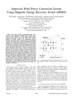
Wind farms were initially installed onshore (Figure 1), and indeed this trend continues. However, in some northern European
countries, a combination of the scarcity of suitable onshore sites with exploitable wind resources and certain favorable characteristics
presented by the sea has led to the installation of offshore wind farms, as shown in Figure 2, which first began to be developed from
1991 onward [3, 8, 11]. The initiative to install offshore wind farms was taken by Denmark, followed by Sweden, Ireland, the United
Kingdom, and The Netherlands. By the end of 2010, the 27 member states of the European Union (EU) were benefiting from a total
installed wind power capacity of 84 278 MW, of which 2946 MW corresponded to offshore installations [5]. According to the World
Wind Energy Association (WWEA), the installed wind power capacity worldwide as of the end of 2009 amounted to 196 630 MW [6].

Figure 1 Whitelee onshore wind farm, Scotland, UK. Courtesy of Iberdrola ().

Figure 2 Horns Rev offshore wind farm, Denmark. Courtesy of Vestas Wind Systems A/S ().


Wind Power Integration

571

However, mean wind energy penetration, that is, the percentage of the demand for electricity that is covered over a long time
period (normally 1 year) in a particular region by electrical energy derived from wind resources, can vary considerably from one
country to another. In some countries this penetration was less than 1%, while in Denmark a figure of around 21% was
obtained [6]. For 2008, the mean penetration throughout the EU was 4.2% [8]. However, according to the European Wind
Energy Association (EWEA) and its reference scenario for 2030, 300 GW of wind power will be installed by that year. It is
estimated that this power will produce 935 TWh of electricity, half of which will come from offshore installations, and will cover
somewhere between 21% and 28% of the electricity demand of the EU [8], depending on the evolution of future power
consumption.
Parallel to the growing numbers of onshore and offshore wind farms which are connected to the high-voltage (HV) electrical
network, there has been an increasing interest in proposals for the installation of ‘embedded’ or ‘distributed’ generation (DG), given
the benefits such a system can offer [12–19]. This type of generation refers to small generators that are normally connected to a
distribution network at medium (MV) or low voltages (LV) rather than to a transmission network at high voltages, which is the
normal situation in centralized generation (CG) systems. The use of DG systems rules out the possibility of including large wind
farms or large hydroelectric plants, but does provide the possibility of using generators powered by renewable energy sources,
emergency generators, and combined heat and power (CHP) cogeneration systems. Among the various options that have been
proposed for DG are the subsystems known as microgrids (MGs) [12, 20].
MGs are small-scale, low-voltage networks which aim to supply energy to small communities. An MG’s generation system is
normally hybrid. That is, it usually comprises generators powered by a variety of energy sources [21–26], both renewable and
conventional, and energy storage devices [27–30]. Such a power system supplies energy to loads that are located in the vicinity
through intelligent coordination of the whole system. These MGs can be designed in such a way that they can normally operate
interconnected to the main network [31] or can operate in stand-alone mode [32].
There are a number of advantages to the integration of wind energy into already existing networks or into those under
development. This chapter will examine these advantages, along with the consequences that the unusual characteristics of this
energy source (i.e., its unpredictable nature and the fluctuations in the power generated) can give rise to in the network to which it is
connected, as well as the effects such integration has on the network’s operational strategies. A presentation is also made of
distributed systems together with an explanation of the benefits of the integration of wind energy into normal interconnected MGs
and stand-alone MGs.

2.18.2 Overview of Conventional Electrical Power Systems
Most existing electrical energy systems in the world have very similar structures regardless of the country in question. They are

basically industrial systems geared toward the generation, transmission, distribution, and supply of electricity [33–38] (Figure 3).
Historically, the generation of electricity has been undertaken at large power production stations. Often, this type of centralized
station is located some distance away from the areas of major consumption, and the energy is supplied to these areas via electrical
networks. Large wind farms and renewable DG systems are connected to these networks by feeding energy into and extracting energy
from them. The resulting power flow caused by these installations can affect both the installations themselves and the power
systems to which they are connected. For a better understanding of the problems associated with wind energy integration, an
introduction to a number of questions related to electrical power systems is given below.

2.18.2.1

Structure of an Electrical Power System

Electrical energy systems can basically be structured into three main blocks: generation, energy transmission/distribution networks, and
loads. A brief presentation of each of these aspects, as well as of control and protection systems, will be made in the following sections.

2.18.2.1.1

Generation

Power stations traditionally convert the energy stored in a primary energy source like coal, oil, nuclear fuel, gas, or a volume of water
at a certain height into electrical energy. The most commonly used technologies are hydro, thermal, and nuclear power plants.
The generation of hydroelectric power (Figure 4) entails the conversion of the potential energy of a volume of water located at a
certain height into kinetic energy in a hydraulic turbine and the conversion of mechanical energy into electrical energy in an
electrical generator. So, hydroelectric power stations require a flow of water and a difference of level in that flow [23, 28, 38–42].
Depending on the method used to control the flow of water, hydroelectric plants can be classified into two basic types: run­
of-river power plants and reservoir power plants. Run-of-river power plants take part of the flow of a river and direct it toward the
turbines. There are a variety of possible configurations, but this type of plant can only allow small controlled flows of water through
the turbines. Reservoir power plants have the capacity to store water by means of a dam and thus control the flow of water through
the turbines and, consequently, the production of electricity.
Thanks to the storage capacity of reservoir power stations, these power stations can be combined with pumping stations to make

pumped storage plants. The pumping stations are responsible for returning to the dam, or the upper reservoir, the water that has
been discharged from the turbines into a reservoir constructed in the lower part of the station. In this way, the surplus energy


572

Wind Power Integration

Central power stations

Substations EHV

V > 145 kV

Transmission
network
Very large
customers

Medium-sized
power stations
Substations HV

36 kV < V < 145 kV

Subtransmission
network
Large
customers

Substations HV/MV

1 kV < V < 36 kV

DG

Distribution
network
Medium
customers

MGs
V < 1 kV

DG

MGs


Small customers

Figure 3 Schematic diagram of the structure of an electrical power system. EHV, extra high voltage.

Figure 4 Cortes de La Muela hydroelectric power station in Cortes de Pallás, Valencia, Spain. Courtesy of Iberdrola ().


Wind Power Integration

573

produced by thermal and nuclear power stations which face certain difficulties in controlling power output can be stored. Likewise,
the surplus variable energy generated by wind farms can also be stored.
Hydroelectric power plants employ various systems and devices for their supervision, control, and protection, depending on the
type of technology employed and the envisaged operating parameters. Smaller hydroelectric power plants (<5 MVA) tend to use
induction generators. However, most hydroelectric power stations operate with synchronous generators. Some of the operating
characteristics of hydroelectric power plants are of particular interest. These plants enjoy a fast start-up response, with start-up times
of just a few seconds. Moreover, they can maintain a practically constant efficiency throughout the power output range, which can
be widely controlled. So, hydroelectric power plants constitute a highly flexible source of electrical generation that can be adapted to
variations in demand. Other advantages include the cost of the fuel and the absence of atmospheric contamination. However,
drawbacks of such plants include the high investment costs, a degree of randomness and constraints in terms of the amount of
primary energy available, and the need to flood extensive areas with its consequent environmental impact.
Conventional thermal power plants convert the primary energy that comes from a fossil fuel (coal, oil, or natural gas) into
electrical energy [23, 34–38, 42–46]. In these power stations, the fuel is burned in a steam boiler. Here, the primary energy is
converted into the thermal energy contained in the steam and gas emissions which are produced in the combustion process and
escape into the atmosphere. A steam turbine (Figure 5) converts the thermal energy stored in the water vapor into mechanical
energy, namely, the rotational movement of a shaft. This mechanical energy is then turned into electrical energy by means of a
generator coupled to the turbine shaft (Figure 6).
As a result of the thermal inertia of the boiler, these power stations are somewhat inflexible in terms of connection and
disconnection. Moreover, control of conventional units is not possible over the entire power output range. In order to guarantee
power generation availability and to improve the system’s flexibility, a large number of units need to be permanently connected
covering the loads, regardless of the power demand. This means that a number of turbines operate under partial load, which is
uneconomical. The use of conventional thermal units to cover demand peaks results in efficiency losses and an important restriction
to optimizing the use of the primary energy source.

Figure 5 Steam turbine at Jinámar power station, Gran Canaria Island, Spain. Courtesy of ENDESA.

Ashes

CO2
Boiler

Water

HighMediumGovernor pressure pressure
turbine
turbine
Steam

Lowpressure
turbine
Generator

Air
Substation

Fuel
Condenser

Figure 6 Schematic diagram of a steam turbine for power generation.


574

Wind Power Integration

One of the advantages of thermal power stations is that, in principle, enough primary energy can be stored to guarantee its
availability for continuous use during a reasonably long period of time. Drawbacks of the system, in addition to those outlined
above, include the cost of the fuel and its contribution to atmospheric contamination.
Conceptually, the turbines employed in gas-fired thermal power stations (Figure 7) are basically the same as steam turbines. The
fundamental difference lies in the fact that the stream which strikes the turbine blades is a mixture of the gases that result from the

combustion of the fuel used, rather than water vapor (steam). The system uses a compressor which introduces air at high pressure
(thereby raising its temperature) into a combustion chamber where it is mixed with the fuel, which ignites without a large increase
in pressure, raising the temperature of the air. The gases thus generated are directed toward the blades of a turbine, causing its shaft
to rotate. This shaft is coupled to an electrical generator (Figure 8). The exhaust gases, usually at a temperature range of 400–600 °C,
are emitted into the atmosphere.
Modern gas turbines used for electrical power generation employ axial compressors and multistage turbines in order to achieve
high levels of efficiency. A number of strategies aimed at improving efficiency have been proposed.
Gas turbines are a little behind hydroelectric plants in terms of start-up times, interruptions, and operational load range. They are
suitable for covering power demand peaks. In just a few minutes, they are able to achieve full output and can respond rapidly to
variations in load demand or unforeseen output losses on the part of other generators. Most gas turbines burn natural gas, which is a
relatively clean fuel. In addition to the relatively low contamination produced, investment costs are lower than those for coal-fired
thermal power plants.
Gas turbines in themselves are not very efficient. This is partly due to the fact that the exhaust gases are still very hot. In other
words, the exhaust gases contain a significant amount of energy which is not being exploited. One strategy to combat this is to
capture the heat of the exhaust gases in a steam boiler and produce steam to drive a turbine and generate additional electricity
(Figure 9). This is the principle behind combined cycle power plants (Figure 10). These plants are capable of achieving efficiencies
of up to 60%. This advantage, along with their modularity and the relatively reasonable investment costs, makes them useful for
covering base demand and peaks.

Figure 7 Gas turbine at Jinámar power station, Gran Canaria Island, Spain. Courtesy of ENDESA.

Fuel
Governor
Air
compressor

Gas
turbine
Combustion
chamber

Generator

Substation
Air
Figure 8 Schematic diagram of a gas turbine for power generation.

Exhaust


Wind Power Integration

575

Fuel
Governor
Air
compressor

Gas
turbine
Combustion
chamber

Generator

Heat recovery
Substation

Exhaust heat

Condenser

To atmosphere
Air
Water
Steam
Governor

Generator

Steam
turbine
Figure 9 Schematic diagram of a combined cycle plant for power generation.

Figure 10 Combined cycle plant in Tarragona, Spain. Courtesy of Iberdrola ().

In conventional power stations, generating units based on reciprocating engines or piston engines are also used. Reciprocating
internal combustion engines are devices that convert the chemical energy contained in a hydrocarbon into mechanical energy
(rotation of a shaft with a certain speed and torque) and into the thermal energy of the waste gases that escape into the atmosphere.
These engines can generate electricity if an electrical generator is coupled to its output shaft, while the waste heat can also be
exploited for thermal applications (cogeneration). These piston engines can be classified into three categories: high-, medium-, and
low-speed engines. The choice will depend on the application. Large engines of low (Figure 11) or medium (Figure 12) speed are
generally the most suitable when it comes to covering the base load. However, high-speed engines are more effective, economically
speaking, for use as a backup service, where there is no requirement to operate over many hours throughout the year. Internal
combustion engines can work well under partial-load conditions. Diesel engines in particular work very well when dealing with falls
in load from 100% to 50%.
Modern-day nuclear power plants (Figure 13), of which there are several types, generate electricity by utilizing the enormous
amounts of energy released when the nucleus of certain heavy elements, like uranium, splits after being bombarded by neutrons in a
process known as nuclear fission [23, 35, 38, 47–51]. The means of exploiting this type of energy is exclusively through the
production of heat, which raises the temperature of a substance such as water, carbon dioxide, or sodium, converting it into steam or

a high-pressure gas and driving a turbine with this pressure to transform the thermal energy into mechanical energy. Connection of
electrical generators to the turbine shafts enables the production of electricity.


576

Wind Power Integration

Figure 11 Low-speed diesel generation unit at Jinámar power station, Gran Canaria Island, Spain. Courtesy of ENDESA.

Figure 12 Medium-speed diesel generation unit at Las Salinas power station, Fuerteventura Island, Spain. Courtesy of ENDESA.

Figure 13 Nuclear power station at Cofrentes, Valencia, Spain. Courtesy of Iberdrola ().


Wind Power Integration

577

Nuclear plants are more capital-intensive than plants which use fossil fuels, but the cost of the fuel is much less. As a result of the
high investment costs and the problems that can arise when changing the reactor’s cooling conditions, it is advisable to use these plants
to cover the base demand operating at maximum availability in order to achieve a high utilization factor of the nuclear energy. The
main drawbacks of nuclear power arise as a result of the dangers associated with breakdowns and the problems involved in the
disposal of radioactive waste. As a consequence, nuclear power plants are the most controversial of all power generating systems.

2.18.2.1.2

Electrical networks

Conventional electrical power generation plants produce power at a voltage between 6 and 25 kV. These relatively low voltages are

not suitable for the transmission of power over long distances due to the losses that occur during transmission. Longitudinal losses
are proportional to the resistance of the medium and the square of the intensity of the current that is circulating. Therefore, the
intensity and/or resistance need to be reduced in order to reduce the losses [34, 35].
The voltage that leaves the power station has to reach the terminals of the consumers. Since voltage drops occur across the
impedance of the network, the impedance of the network or the intensity of current needs to be reduced in order to reduce the
voltage drop. For this purpose, large transformers are used, which raise the voltage to hundreds of thousands of volts, transmitting
the same power but reducing the current [34, 35, 37, 38]. On lowering the intensity and increasing the voltage, losses as a result of
the Joule effect are reduced quadratically, while the voltage drop is linear [35].
Extra-high-voltage lines transmit the energy produced by the power generation stations to high-voltage substations – the starting
point of the so-called subtransmission networks (Figure 3). These networks operate at a lower voltage than the transmission
networks and, in turn, supply the local networks, known as distribution networks, via substations that reduce the high voltage to
medium voltage. The distribution networks usually have a distinctively radial configuration for the purpose of supplying energy to
the medium- and small-sized consumers spread out throughout the area and connected, respectively, to medium and low voltages.
Medium-sized consumers are generally the large industries, while the small-sized consumers tend to be represented by domestic
loads, businesses, and small factories. In order to cover their particular energy requirements, large-sized consumers are usually
connected to the high-voltage network (Figure 3).
Electrical networks, fundamentally comprising lines and substations, were initially used to connect the production and
consumption centers of a particular region. Gradually, however, from the end of the nineteenth century to the present day, these
networks have found themselves hooked up to other networks of nearby areas until the networks have grown to cover the geography
of each country [35]. Figure 14 shows an outline of the transmission network map of the Spanish mainland system. According to
Red Eléctrica de España (REE), the Spanish transmission system operator (TSO), Spain’s transmission system in 2009 was
34 754 km long, with 3385 substation positions and a transformation capacity of 66 259 MW. Indeed, given the economic
advantages presented by network interconnection, some continents now have network interconnections between several countries,
with the consequent creation of enormous and complex supranational meshed networks.
Most networks work with alternating current (AC), though there are a few exceptions in high-voltage energy transmission (e.g.,
direct current (DC) transmission may be more convenient when the aim is to connect production and consumption centers
separated by considerable distances) [35]. So, when operating at the same rated frequency and with all the synchronous generators
in phase, it is possible for the energy produced in an area of one country to be transmitted beyond its frontiers and shared with other
areas of the country or with other countries. One of the advantages offered by a robust and secure meshed network is supply
continuity, since the various substations can be fed from a number of directions. The feasibility of reducing the reserve capacity

required to cover demand peaks also constitutes an added value. Another advantage lies in the possibility of reducing the spinning
reserve, namely, the power that has to be connected, but without a load, to cover unforeseen increases in demand. The way that

PORTUGAL

FRANCE

Generation system
Substation

Figure 14 Spanish mainland’s electricity transmission network map. Courtesy of REE ().


578

Wind Power Integration

Figure 15 High-voltage tower. Courtesy of Iberdrola ().

these interconnected networks function sees the reserve capacity shared out between different generation centers in such a way that
there is mutual support against network disturbances. Market systems can decide how the power injected into the network is to be
shared out between the different power generation stations at any given moment.
Aerial power lines (Figure 15), which generally consist of steel-reinforced, stranded aluminum alloy cables, are sized according
to the maximum operating voltage, the power to be transmitted, the distance involved, and the location of the starting/end points
and other interconnection nodes [34, 35]. The aim is to achieve a design that, from both an electrical and a mechanical point of
view, generates the least longitudinal and transverse losses in the transmission of the energy and minimizes the investment,
operating, and maintenance costs. Longitudinal losses are primarily due to the Joule effect, while transverse losses are the result of
the corona effect. The Joule effect and the corona effect [37] are related to the operating current and voltage, respectively.
Fiber-optic cables of the telecommunications network can also be housed inside the high-voltage cables. Spain’s TSO, respon­
sible for the high-voltage network, currently has a network of more than 21 300 km of fiber-optic cable and around 19 000 devices

to provide telecommand, telecontrol, and teleprotection services [52].
The substations [53] act as network nodes and, in their most basic configuration, comprise thick bars to which the electrical lines
are interconnected. They can, however, be configured in very different ways, each one of which gives the substation different
characteristics in terms of reliability, operational flexibility, cost, and so on.
Substations (Figure 16) can be classified according to their use, and they fulfill a variety of functions. One of those functions is to
serve as an interconnection point for the power lines, directing the power flow toward different geographical regions in such a way

Figure 16 Substation at La Vall D’Uxió, Castellón, Spain. Courtesy of Iberdrola ().


Wind Power Integration

579

that the flow of power generated in the various power generation stations can be controlled in accordance with the country’s energy
policy or market conditions. Another function can be as a transformation center which carries out interconnections at different
operating voltages. This function also includes raising the outgoing voltage of the transformation centers. A third function is that of
housing the various elements of protection, cut-out, and switching.
The equipment of a substation comprises power transformers, devices used to connect and disconnect electrical circuits,
measuring and protection transformers, protection relays, and so on, depending on its configuration.
Among the devices used for the connection and disconnection of electrical circuits are automatic switchgear and isolators.
Automatic switchgear is designed to open and close a line along which an abnormally high current circulates as a consequence of,
for example, a short circuit. The job of the isolators is not to cut off any current, but rather to electrically isolate in a visible way the
damaged area once the current along the line has been cut off as a result of the activation of a switch. Measuring and protection
transformers, usually of current or voltage, are used to power the measuring instruments, relays, and other equipment, including the
communications system. Measuring devices detect faults, and the protection equipment decides what switch needs to be activated to
clear the fault. For this reason, protection systems need to be selective, reliable, and sensitive enough to operate under
minimum-fault conditions in the system area for which it is responsible and must be able to act with a speed appropriate to the
type of fault that needs to be cleared. Selectivity in this case is related to the capacity to clearly recognize the type of fault and to
minimize the size and extent of the interruption. Reliability indicates the capacity to operate exclusively when a fault condition

arises.
Though the interconnection of networks does present economic advantages, the intensity of the current increases when a short
circuit occurs in a system. Disturbances caused by a short circuit can extend to systems that are interconnected to it. So, for a network
to fulfill its mission and guarantee its operation in secure and safe conditions, it must be equipped with appropriate measuring,
protection, and control equipment.

2.18.2.1.3

Loads

Power systems have to cover the demand for electricity that may come from a number of consumer categories: industrial, domestic,
commercial, and so on. Instantaneous power demand is typically a variable parameter that depends on the electricity requirements
of the consumer at any given moment [23, 35–37, 54]. The profiles represented by the power demand as a function of time
(typically 24 h) are known as load curves. The area enclosed by a load curve and the time axis represents the energy consumed in the
period under consideration.
The load curve for each consumer category usually has its own distinctive characteristics [18, 23]. Some may display clearly
noticeable demand peaks and troughs, while others may be flat. For example, the maximum domestic sector consumption tends to
occur when people are at home and are using their electrical household appliances. This happens usually during mornings and
evenings and at weekends. By contrast, the domestic sector’s minimum consumption tends to be during the rest of the day and at
night. Electricity consumption is also extremely dependent on the weather and climate of a particular region, which affect the
amount household appliances consume for cooling or heating purposes. Industrial consumption tends to display a more stable
profile than domestic or commercial consumption.
By superimposing the different load curves of the various consumer types, the electrical system’s load curve is obtained. These
load curves can be represented for different time periods. That is to say, they can be daily, weekly, monthly, or annually. It should be
mentioned that fluctuations in total demand are less than those corresponding to an individual load. In other words, demand
aggregation gives rise to a smoothing effect of the load curves. This is due to the different load profiles of the various consumption
sectors and the random component of demand. As a result, the variance of total consumption is less than that of any one individual
consumer type.
Figure 17 shows the total demand curve for 14 and 15 February 2010 (a Sunday and Monday, respectively), in the Spanish
mainland system. The variability of demand over time can be observed together with the hourly intervals in which the peaks and

troughs took place. Figure 18 shows the evolution of the peaks and troughs of the daily demand curves recorded during 2009. The
influence of weekends and holiday and seasonal periods can be observed.
Meanwhile, each point of the so-called load–duration curves indicates, on the x-axis, the accumulated time in which the system’s
power demand was higher than the value indicated on the ordinate axis (Figure 19). These curves, like the load curves, can be
represented for different time periods: weekly, monthly, or yearly.
Though it depends on the nature of the loads, that is, whether they are resistive or inductive, the overall power demand has an
active and a reactive component. Active power is the power converted into physical power. Reactive power helps create the magnetic
field which certain loads require. So, there is a variation of these components in the daily evolution of power demand. With regard
to reactive power, it should be mentioned that aerial power lines, depending on their load, generate or consume reactive power.
Transformers, on the other hand, always consume reactive power.
The electrical demand of the loads, unlike the other components of a conventional electrical generation system, cannot be
controlled and displays a high degree of randomness. This random behavior can be modified to a certain extent through the use of
demand-side management techniques aimed at rationalizing electrical energy consumption [55–57]. Some loads, normally known
as deferrable loads or interruptible loads, can postpone their connection to the network within certain time intervals. Loads that can
feasibly be temporarily interrupted include those that have thermal inertia (air conditioning, heating, etc.), certain water pumping
applications, and sea or brackish water desalination plants [58–60]. Likewise, the establishment of electricity tariffs that depend on


580

Wind Power Integration

46 000
44 000
PO
RT
UG
AL

42 000

Power demand (MW)

40 000

Sunday

FRA

NCE

SPAIN

38 000
36 000
34 000
32 000
30 000
Monday

28 000
26 000
24 000
22 000

0

2

4

6

8

10

12
14
Hours

16

18

20

22

24

Figure 17 Power demand curves of the Spanish mainland electricity system for 2 days in February 2010. Courtesy of REE ().

45
AL

FRA

RT

UG

NC

Power demand (GW)

Maximum power demand

E

SPAIN

PO

40

35

30

25

20
Minimum power demand
15

Jan

Feb Mar

Apr May Jun

Jul

Aug Sep

Oct

Nov Dec

Months
Figure 18 Maximum and minimum power demand curves for 2009 in the Spanish mainland electricity system. Courtesy of REE ().

45

Peak load

40


Load (GW)

35

Intermediate load

30
25
20
15

10

Base load

5
0
0

1000

2000

3000

4000

5000

Hours
Figure 19 Example of a load–duration curve.

6000

7000

8000

8760

Wind Power Integration

581

the amount consumed and the time of consumption (via the use of time bands) can have the effect of persuading consumers to react
to the price of the energy used and alter their consumption habits accordingly.
In order to be able to carry out both the planning and operational tasks of an electrical system, short-term demand has to be
estimated in all situations. The use of predictive models based on time series [61, 62] and models that employ data mining
techniques, such as neural networks [63], has been proposed to estimate short-term demand and employ it in electrical system
operational tasks. These models take advantage of certain behavioral traits that are observed in the evolution of demand, which have
been mentioned above, namely, the relationships that exist between the demand and parameters such as type of day, time of the
day, climate and atmospheric conditions, type of user, and geographical location.
Electricity operators have developed expert systems for the forecast of daily and hourly demand to help in their operational
decision-making [52].

2.18.2.2

Operational Objectives of an Electrical Power System

The operational objectives of electrical power systems can be synthesized into two fundamental priorities, namely, guaranteeing
continuity of supply so that demand is covered with the required quality and, within the restrictions imposed by this objective,
ensuring that the system is run in the most economic way possible [62, 64, 65].
Guaranteeing continuity of supply requires the establishment of security criteria in the operation of the electrical system. For this,
a series of parameters must be controlled that enable supervision of the status of the electrical system. These parameters are the
frequency, the voltages at the network nodes, and the load levels in the various elements of the transmission network that the system
operator manages, namely, the lines and substations.
The control centers (Figure 20) [9, 52] manage the information they receive in real time from the power generation centers and
the network via an extensive telecommunications network. Studies that guarantee security of the electrical system are carried out
using this information.
Security depends on the robustness of the system in the face of predefined contingencies. For example, the contingencies that are

normally considered are (1) single outage of any element in the system; (2) simultaneous outage of double-circuit lines that share
towers over an extensive section of the line path; and (3) in special situations, the outage of the largest generator unit in the area and
of one of its interconnection lines with the rest of the system [33].
The system must have the capacity to maintain the control parameters within certain preestablished admissible limits in the face
of changes in demand and contingencies that may arise. Given the inherent uncertainty in relation to some contingencies, when the
term ‘security’ is used, it often refers to a measure of short-term operational reliability.
The second objective of electrical power systems is related to what is known as the economic dispatch [33, 62], that is, the
method of dispatching the available generation resources to supply the load on the system in such a way that the total generation
cost is minimized.

2.18.2.3

Operating States of an Electrical Power System

A balance must be achieved at all times in the operation of electrical systems between generation and demand without overloading the
system. The function of the system operator lies in ensuring that this balance is always maintained. For this purpose, the operator needs
to be able to forecast demand and supervise the generation and transmission installations in real time. If the system gets out of balance,
the operator orders the production centers to adjust generation so that it can be adapted to the variations in demand. However,
depending on the conditions in which the power system finds itself, it can be run under different operating states [33, 66, 67].
In the normal operating state, in addition to the prerequisites that there exist a balance between generation and demand and that
the restrictions imposed on certain variables be met, a specific security level is also contemplated. That is, the normal operating state
is also characterized by reserve margins, in relation to both the transmission system and the power generation system. Typically, a
system will find itself under the normal operating state for a high percentage of the time [68] (Figure 21).

Figure 20 Electricity Control Center of REE, CECOEL. Courtesy of REE ().


582

Wind Power Integration

NORMAL OPERATION
Generation-demand balance

Variables within limits

B

RESTORATION
B

V

Generation reserves

V

Restoration control

Preventive control

R

Loss of reserves

R

Restoration control

ALERT

OPERATION

Load shedding

EMERGENCY
OPERATION
B

V

R

Emergency control
B

V

R

Contingency

Figure 21 Schematic diagram of the operating states of an electrical power system.

If the levels of security fall, whether as a result of an increase in load or due to the probability that some disturbance will occur,
then the system reliability gets reduced. When the level of security falls below a specified limit, even if the demand is covered and the
operating limits imposed on the variables are not breached, the system finds itself in the state known as ‘alert’.
In alert state, any disturbance caused by the evolution of demand or the presence of a contingency could result in the operating
variables being outside their established ranges. If such a situation arises, the system changes to emergency state.
When a system is in emergency state, it has to make urgent use of corrective measures required to avoid the system losing its
integrity and collapsing. Among the measures that can be used to ensure that the values of the variables return to admissible

operating intervals is the temporary suspension of the supply to the users. That is, a load shedding is performed.
In some countries, automatic load shedding is undertaken following the guidelines of the Union for the Coordination of
Transmission of Electricity (UCTE), which has established the load percentages to be disconnected depending on the frequency of
the system. However, it must be pointed out that from 1 July 2009 onward, the European Network of Transmission System Operators
for Electricity (ENTSOE) [69] took over all operational tasks of the six existing TSO associations in Europe, including the UCTE.
There are also nonautomatic, selective load shedding mechanisms designed to avoid loss of demand in alert or emergency
situations. Both types of shedding try to avoid the disconnection of highly sensitive loads, such as hospitals and radio and television
services. Likewise, as mentioned in Section 2.18.2.1.3, there can also exist load interruption services. In Spain, this service can be
offered by consumers who acquire the energy from the production market [52]. The system operator, depending on the category of
the load interruption service, can interrupt the energy supply to the consumers during certain time periods. In practically all
the service categories, the consumers must be given prior notification.
Action must be taken to restore the system to the normal or alert status. In problematic situations, operational objectives of a
technical nature take priority over economic ones.
From the consumer’s point of view, optimum quality of the electricity supply is determined by the uniformity of the voltage,
with a pure sinusoidal wave at a constant frequency and effective value. The quality of the supply will be affected by disturbances
that modify these characteristics. Sine wave purity is becoming increasingly relevant as a result of the demands of the recipients. The
waveform can be distorted by both the generation itself and the actual recipients of the electrical energy. The problems related to
waveform quality are usually tackled at a local level. However, supervision of the frequency and effective value of the voltage is
usually dealt with by a centralized and hierarchical control structure.
In order to better understand how electrical energy systems function, something which will be useful when it comes to analyzing
the impact of wind energy integration into the systems, the following sections will provide a brief description of (1) active power
and frequency control and (2) reactive power and voltage control, though to a certain extent both types of control are interrelated.

2.18.2.3.1

Active power–frequency control

The rated frequency used in European and African countries is 50 Hz. This frequency is also used by the vast majority of countries in
the Middle East, Asia, Australia, and the Pacific Islands. However, in the United States, Canada, and most Central and South
American countries, the frequency used is 60 Hz.

The frequency of an electrical system is closely related to the equilibrium that exists between the power supplied by the
generation system, the power consumed by the loads, and power losses. When there occurs a deviation in this power balance,
the control system acts to reestablish it following a hierarchical procedure organized into three stages: primary, secondary, and
tertiary control [52, 65, 70]. Each of these levels operates over different time margins and involves areas of greater or lesser size of the
whole electrical system.


Wind Power Integration

583

If the power demand increases sharply or a generator fault occurs, the primary control stage must be immediately available to
provide the generation power required to reestablish the system’s power balance. This additional generation power is provided
initially by making use of the kinetic energy stored in the rotating elements of the power generation units, which are able to provide
full output power for a few seconds, and following this by intervention of the turbine and engine speed governors.
The kinetic energy depends on the inertia of the rotating masses and the rotational speed. The rotational speed of the
synchronous generators of an electrical system is proportional to the frequency of the voltage. So, a deviation from the active
power balance leads to changes in the rotational speed of the generators and, consequently, in the frequency of the system.
After a certain delay, while the system responds to the release of the stored kinetic energy, more significant amounts of energy can
be supplied to restore the active power balance. This supplementary energy is achieved through the intervention of the systems that
regulate the opening of the valves that control engine fuel input, the flow of water in hydroelectric plant turbines or the flow of gas
or steam in thermal power plant turbines (Figure 22). As the engines and turbines are mechanically coupled to the generators it is
possible to regulate the power that the latter generate by controlling the mechanical power output of the former. When a reference
power level is either not reached or exceeded, the turbine and engine governors adjust the valves to increase or decrease mechanical
power. It should be mentioned that some loads are sensitive to frequency changes and vary their power demand accordingly.
The participation of generators in restoring the power balance depends on their power–frequency characteristic. This character­
istic depicts the variation in frequency when the power generated by a machine changes from zero to its rated value. This
relationship can be approximated to a straight line whose slope, of negative sign, is the constant of the governor. This constant is
what determines the characteristic of the governor in continuous operating conditions (steady state) and is known as the generator
speed droop. Speed droop is expressed in hertz per megawatts, and typical values are in the range of 4–6%. The point where the

straight line intercepts the frequency axis is known as the set point. The governor allows the system operator to adjust the set point in
such a way that the mechanical power output varies without modifying the frequency.
Figure 23 shows the power–frequency characteristic which corresponds to a generator with a specific regulation constant,
operating at two different set points. However, the primary control does not modify the set point; rather, the variation in mechanical
power is obtained by varying the frequency.

Governor
valve

Exhaust
Turbine

Steam
Flow

Valve
control

Speed
sensing
device
Synchronous Threephase
machine
grid

Rotational
speed Electrical
power
Load

Substation

frequency
control

Frequency
Measurement
device
Reference power

Figure 22 Schematic diagram of the frequency control system of a synchronous generator.

f
B
Frequency (Hz)

Set points

A
Δf/ΔP

System frequency (fS)

Δf/ΔP

P
PA

PB

Generator power (MW)
Figure 23 Active power–frequency characteristic of a generator with two set points (A and B). PA, power supplied by the generator with set point A;
PB, power supplied by the generator with set point B.


584

Wind Power Integration

f

Unit A set point

Frequency (Hz)

Speed droop unit A
Unit B set point

Speed droop unit B

System frequency (fS)

P
Output power (MW)

Output unit A
Output unit B
Figure 24 Schematic diagram of load distribution between two generators in parallel with different speed droops.

When there are various generators of different rated powers working in parallel with different speed droops, the contribution

each one makes will depend on the value of its speed droop. A unit with a lower speed droop will contribute to the primary
regulation a higher percentage of power with respect to its rated power, while a generator with a higher speed droop contributes
a lower percentage of power. Figure 24 shows load allocation between two generators with different speed droops. If several
units in parallel have the same speed droop, all of them will contribute to the primary control proportionally to their rated
power.
Primary control, which acts at a local level, enables restoration of the balance between power generated plus losses and
power demanded. The primary control must complete its intervention within 15–30 s of the instant when the imbalance takes
place. This time will depend on the magnitude of the imbalance. The primary control ensures that the frequency is never outside
the acceptable range. However, this control is unable to prevent the frequency from remaining deviated from the nominal or
rated reference frequency. In addition, the load increase allocation among the generators does not have to maintain the power
flows that have been scheduled. In some countries, like Spain, primary control is an obligatory and unpaid complementary
service that must be provided by connected generators. In Spain, primary control of generating units must allow a speed droop
such that the generators can vary their load by 1.5% of their rated power [52].
The secondary power–frequency control acts on a zonal level, where the frequency in each of the neighboring production zones
is uniform. This control level allows the defects of the primary control to be corrected, though it is slower-acting. Commencement of
secondary control intervention should not be delayed for longer than 30 s. The automatic generation control (AGC) is responsible
for this intervention level, and its actions are centralized.
As has been mentioned, it is possible to modify the reference power of the generators. That is, it is possible to change the set point
in the power–frequency characteristics. This action entails vertical movement of the power–frequency characteristic, as can be seen
in Figure 23.
Through determination of the reference power that has to be produced by each generator which intervenes in the secondary
control, the frequency error can be corrected in a stable manner, thereby contributing to maintaining the frequency in that particular
zone or area. In addition to covering the demand of the area, secondary control, which is performed by the system operator, must
maintain the scheduled energy exchanges. The control strategy defines for each area an error signal known as the area control error
(ACE). The reference power variation allocated to each of the generators that participate in the secondary control has to be
proportional to the integral of the ACE. That is, the error signal is an input variable of an integrator. Its purpose is that the
mechanical power variation of the generators is modified in such a way that the area error tends to zero in steady state. The gains of
the integrator are determined with control stability criteria.
In the participation of the different generation systems in frequency control and demand variation control, several strategies can
be used based on speed of response, nondiscrimination of generator type, and so on. The intervention time of the secondary control

reserve is usually limited and should normally be no greater than 15 min.
The reserve power that must be maintained to undertake secondary control is determined by the system operator. In the Spanish
mainland electrical system, the recommendation of the UCTE is normally taken as the point of reference. In Spain, the secondary
control service is optional and paid for through market systems [52].
Tertiary control operates over a more extensive range of the electrical system, simultaneously regulating the frequency and
voltages following economic and security criteria [33]. The purpose of tertiary control is restoration of the secondary control reserve
to make it available again. In general, tertiary control works with generators that may or may not be coupled and must act within a
time margin of between 10 and 15 min, and its reserves must be able to be maintained for some hours.
In some countries, tertiary control is a complementary service which is optional and paid for through market systems.


Wind Power Integration

2.18.2.3.2

585

Voltage control

The purpose of voltage control is maintenance of the effective value of the voltages in the network within acceptable limits [33, 52,
64, 65, 68]. There is a close relationship between the reactive power flow between two network nodes and the difference between the
effective voltage values at these nodes. Reactive power variations entail voltage variations. So, the control system has to be constantly
working to correct voltage deviations. There must also be reactive power reserves available to resolve any voltage incident that might
take place.
A variety of devices can be used to control the voltage. These include static compensators, synchronous compensators, and
synchronous generators [71].
Capacitor and/or reactor banks constitute static compensators that inject or consume reactive energy into/from the nodes where
they are connected. The voltage is discretely modified via connection and disconnection of these devices. Mechanical connection is
performed through relays and electronic connection through thyristors.
Static compensators consisting of fixed-capacity condensers and adjustable coils can be used for continuous regulation of the

reactive power injected or consumed into/from the network. This device is known as a thyristor-controlled reactor-fixed capacitor
(TCR-FC; Figure 25).
Thanks to advances in power electronics, the pulse-width modulation (PWM) technique is being used more and more
commonly in power electronic systems [72–76]. Indeed, it can be stated that the PWM technique has opened up a whole new
field in reactive energy compensation methods.
Static compensators (STATCOMs) normally use the PWM technique. The STATCOM (Figure 26) is a voltage-sourced converter
(VSC) system that generally uses gate turn-off thyristors (GTOs) or insulated gate bipolar transistors (IGBTs) combined with diodes
enabling application of the PWM technique. The frequency at which the switches operate can vary depending on the power of the
system to which the STATCOM is connected. Thus, the STATCOM behaves as if it were a synchronous capacitor, consuming or
absorbing reactive power continuously, but without storing energy to compensate.

AC three-phase grid

Control
SCR

Reference
reactive
power

Fixed
capacitor

Variable
inductance

Fixed
capacitor

Inductance

Equivalent model
Figure 25 Schematic diagram of a TCR-FC. SCR, silicon-controlled rectifier.

AC three-phase grid

GTO

Coupling
transformer
Diode

Fixed
capacitor

Inductance

Variable
controlled
voltage
source
Equivalent model

Figure 26 Schematic diagram of a STATCOM.


586

Wind Power Integration

Reference voltage
Governor
valve
Turbine
Steam
flow

Automatic
voltage
control

Measurement
device
Voltage

Excitation
system
Threephase

Synchronous
machine

Substation

Exhaust
Figure 27 Schematic diagram of the voltage control system of a synchronous generator.

Control of static compensators, in the specific case of voltage regulation in an electrical power system, is carried out by means of
a closed loop similar to that of the governors used in synchronous generators. The bar voltage is compared with a reference voltage.
The error passes through a proportional–integral governor, which generates the firing angle required to obtain the desired voltage.

A synchronous compensator, also known as a synchronous capacitor, is a synchronous machine whose shaft is not coupled to
any mechanical load. It consumes and generates reactive power when underexcited and overexcited, respectively. There are a
number of advantages to this device when compared with static compensation devices, including continuous voltage regulation
without electromagnetic transients. Another advantage is that they do not introduce harmonics into the network, nor are they
affected by them. Likewise, they do not generate problems as a result of electrical resonance.
Like frequency control, voltage control is also undertaken at hierarchical levels [33]. The primary control aims to maintain a
voltage set point at a particular system node. The synchronous generator constitutes the most characteristic element in primary
control of voltage. Synchronous generators, which can modify their active power as described in Section 2.18.2.3.1, are also capable
of modifying their reactive power. Control of the latter is automatic and is achieved via regulation of the generator excitation current
(Figure 27).
Automatic voltage regulation (AVR) acts within a very few seconds, and its objective is to control the generated reactive power
and/or maintain the voltage at the generator terminals. A sensor measures the voltage at the generator terminals, corrects it, and
compares it with the desired voltage.
While primary voltage control is local in scope since the information it uses is local, secondary control [33, 70, 77, 78] is
responsible for the voltages of a set of representative nodes of an area or region, known as pilot nodes. Secondary control
coordinates the voltage governors of the area’s generators and, like primary control, functions automatically.
Tertiary control, as has been mentioned, is a combined control of frequency and voltage. It is generally nonautomatic and uses
information from the whole system to determine the reference values of the pilot nodes.

2.18.3 The Distinctive Characteristics of Wind Energy
Electrical energy generated using wind as the energy source displays some distinctive characteristics, which distinguish it from the
power generated by the conventional energy sources described in Section 2.18.2. In this respect, the most notable features of wind
energy are its temporal and spatial unpredictability and variability, the impossibility of directly storing the primary energy, the
abundance of the resource in many places in the world, and its renewable and noncontaminating character.

2.18.3.1

The Unpredictability and Variability of Wind

The power of wind on the Earth is a consequence of solar radiation [79–81]. On a planetary scale and due, among other factors, to

the shape and position of the Earth with respect to the Sun, there exist insolation differences between different areas of the planet.
Broadly speaking, the thermal differences that occur, combined with the rotation of the Earth with respect to its own axis, give rise to
the displacement of masses of air. Such displacement or the large-scale movement of air is known as atmospheric circulation.
These global winds are affected by the presence of the continents and water masses that shape the Earth’s surface and by the
movement of the planet with respect to the Sun. The circulation of these air masses will also be influenced by local thermal and
climate effects as well as by the orography of the region. Thus, wind characteristics depend markedly on geographical location.
Because of the influence of orographic features, the wind speed in one area can differ substantially from that in another just a few
kilometers away.


Wind Power Integration

587

Figure 28 shows, by way of example, the variation in daily mean wind speeds during the month of August, 2005, at two
anemometer stations on the island of Gran Canaria (Canary Island Archipelago, Spain) installed 10 m above ground level and
separated by a distance of approximately 34 km. The mean wind speed for that month differs by about 36.6%.
The considerable number of variables that can affect the movement of air masses makes the wind unpredictable and, over a wide
range of scales, means that its behavior is both temporally and spatially variable. The wind shows variations from a scale of seconds
to interannual timescales. That is, the mean wind speed of a site can vary from one year to another. Figure 29 shows, by way of
example, the mean interannual wind speed variation over a 10-year period at an anemometer station installed 10 m above ground
level on an island in the Canary Archipelago.
Significant changes can also be observed from one season to another and, indeed, from one month to another during the same
year. Figure 30 shows the monthly wind variation at an anemometer station on the island of Gran Canaria. It can be seen how, given
its geographical location (between latitudes 27°37′ and 29°25′, subtropical, and longitude 13°20′ W of Greenwich), the frequency
of the trade wind regime is very high during the summer months, with the highest wind speeds occurring during that season.
Normally, the wind behaves differently in the Northern Hemisphere, with the summer months seeing the lowest wind speeds.
Similarly, wind speed can vary from one hour to another over the course of a day.

18

16
Anemometer station B

Wind speed (m s–1)

14
12
Mean (B) = 9.54 m s–1
10
8
6
4

Mean (A) = 6.98 m s–1

Anemometer station A

2
0
1

3

5

7

9

11

13

15 17
Days

19

21

23

25

27

29

31

Figure 28 Mean daily wind speed variation during the month of August, 2005, at two anemometer stations on the island of Gran Canaria, Spain.

7.0
6.5
Mean = 5.97 m s–1

Wind speed (m s–1)

6.0
5.5

5.0
4.5
4.0
3.5
3.0

1999

2000

2001

2002

2003

2004

2005

2006

2007

2008

Years

Figure 29 Mean interannual wind speed variation recorded 10 m above ground level at an anemometer station on the island of Gran Canaria, Spain.

588

Wind Power Integration

14

Wind speed (m s–1)

12
10
Mean = 7.36 m s–1

8
6
5
4
0

Jan

Feb

Mar

Apr

May Jun Jul Aug Sep
Months

Oct

Nov Dec

Figure 30 Evolution of the monthly wind speeds during 2003 at an anemometer station on the island of Gran Canaria, Spain.

9

Wind speed (m s–1)

8

7
Mean = 6.3 m s–1
6

5

4

3
1

2

3

4

5

6

7

8

9 10 11 12 13 14 15 16 17 18 19 20 21 22 23 24
Hours

Figure 31 Average daily wind speed evolution at an anemometer station in the Canary Archipelago.

Figure 31 shows, by way of example, the substantial variations observed in the mean hourly wind speed on a day timescale at an
anemometer station installed near the coast of an island in the Canary Archipelago. It can be seen how the wind displays very
high-speed values during the day and lower ones at night. This behavior is the result of the different effects of the heating of the
surface of the land during the day and of the sea breezes.
It is usually accepted that the random variations seen in periods ranging from 1 s to approximately 10 min represent turbulent
wind speed variations. Figure 32 shows the wind speed variation recorded over a 2 h period at an anemometer station located in the
Canary Archipelago. The values for each second and the means for each 10 min can be seen.

2.18.3.2

The Variability of Electrical Energy from Wind Sources

The power that a wind turbine extracts from the wind is proportional to the air density, the rotor swept area, the power coefficient, the
power transmission system efficiency, and the cube of the wind speed [1, 82–84]. The power coefficient is a function of the tip speed ratio
and the pitch angle [82–84]. Air density varies with pressure, temperature, and humidity [85]. However, given the more striking variations
in wind speed and its cubic influence, it is wind speed variations that can give rise to the most significant power fluctuations of a turbine.

Wind Power Integration

589

25
10 August 2009

23

10–12 h

Wind speed (m s–1)

21
19
17
15
13
Means for each 10 min

11
9
7
5

0

10

20

30

40

50

60

70

80

90

100 110 120

Time (min)
Figure 32 Evolution of wind speed recorded each second, over a 2 h period, 40 m above ground level at an anemometer station on an island in the
Canary Archipelago.

Partial load

Full load

Electrical power

Maximum power output

Cut-in wind speed

Cut-out wind speed
Rated wind speed

0
0

Wind speed

Figure 33 Typical power curve of a wind turbine.

There are different control systems that can be used for wind energy conversion systems (WECSs) [3, 8–10, 82, 86–88]. The
intervention of these control systems enables regulation of the electrical power generated by the wind turbine.
Figure 33 shows a typical power curve for a modern pitch-regulated wind turbine. This curve represents the mean performance of
the wind turbine. Oscillations and deviations from the mean values will appear in the event of significant turbulence. Likewise, the
local orography and wake caused by nearby turbines will distort the power curve provided by the manufacturer. Two clearly
differentiated areas can be observed in Figure 33. One area lies between the cut-in wind speed and the rated wind speed and the
other between the rated wind speed and the cut-out wind speed. At the rated wind speed, the electrical generator of the wind turbine
will produce its maximum power output. When the wind turbine is operating in the first section of its power curve, it is said to be
working in the partial-load range. However, if the rated wind speed is exceeded, then the machine is said to be operating in the
full-load range. If the wind speed exceeds the cut-out wind speed for a few seconds, then the turbine stops and, therefore, no longer
produces energy. Likewise, the wind turbine has no output for wind speeds below the cut-in wind speed.
Figure 34 shows the power produced by a wind turbine installed in a wind farm in the Canary Archipelago over a 2-day period. It
can be deduced from the figure that wind speed fluctuations in the partial-load range of a single wind turbine can give rise to large
fluctuations in its electrical power output. In the full-load range, the power curve displays a constant mean performance and is not
affected much by wind speed variations.
The timescale of wind speed variation has a significant effect on the power output fluctuation of the wind turbine. If the spectra of
wind fluctuations are analyzed at a particular site from micro- to macrometeorological range, it can be seen how the kinetic energy of
the horizontal wind speed is distributed as a function of the variation frequency of that wind [89–93]. Regardless of the site where the
spectral analysis is conducted, a valley or spectral gap can typically be observed, which is bounded by one peak at around 1 min and

590

Wind Power Integration

900

18

800

Power

Wind speed

16

1000

500
850 kW

12

800

10

400

600

Power (kW)

600

14

Power(kW)

Wind speed (m s−1)

700

300
400
200

200
8
0

5

0

6
0

4

8

12

16

20
10
15
Wind speed (m s−1)
20

24
Hours

28

32

100

25

0
36

40

44

48

Figure 34 Variation of the electrical power generated by a wind turbine over 2 days at a wind farm in the Canary Archipelago.

another peak at around 12 h. There is normally a third peak in the region of several days. The first peak is the consequence of turbulent
wind fluctuations, the second corresponds to diurnal wind variations, and the third is normally attributed to the passage of
anticyclones and depressions. So, the observed spectral gap separates the daily wind speed variations from turbulent variations.
Within this spectral gap, the interval that ranges between 10 min and a few hours usually reflects a low wind energy content.
Turbulent wind fluctuations which occur on a scale of seconds or minutes can generate substantial deviations in the power output
of a single wind turbine with respect to its mean value. These rapid fluctuations in the electrical energy generated by a wind turbine can
have a harmful effect on the quality of the energy and, therefore, on the electrical system to which the turbine is connected. It should
also be mentioned that the energy production loss of a wind turbine as a result of the high-wind hysteresis effect [87, 93] depends,
among other factors, on the level of turbulence. High-wind hysteresis is basically the turbine’s control system lag between shutting
down when the cut-out wind speed is exceeded and restarting. The reconnection speed is normally 3–4 m s−1 lower than the cut-out
speed. The harm that wind turbulence can cause to the quality of the energy generated and its impact on losses due to the high-wind
hysteresis effect depend to a large degree on the level of the technology installed in the wind turbine.
Knowledge of the short-term behavior of the wind is of vital importance in the operation of electrical systems, whereas monthly,
seasonal, and interannual behavior will have an impact on, among other questions, the planning of the electrical system.

2.18.3.2.1

Effect of wind turbine aggregation on wind power variability

The power output fluctuations of a single wind turbine, as described in the previous section, could cause significant problems in
terms of the integration of the wind power into an electrical power network if the energy generated by each of the various turbines
that make up the wind farm behaved in an identical manner.
The total power output of a wind farm is the summation of the output of each of the wind turbines that compose it. However, since
the wind speeds that strike the rotors of the different wind turbines on a wind farm are generally not identical, the power output

fluctuations of each wind turbine are different. As happens with demand aggregation [94], the total power output fluctuation of the
wind farm is dampened or smoothed out. That is, the overall fluctuation is less than the individual fluctuations [8, 93, 95].
Figure 35 shows the power output of a wind farm installed in the Canary Archipelago over a 2-day period. The wind farm has
nine wind turbines, and the power variation over this period was on the order of 31%. Also shown in the figure is the power output
of the turbine with the highest variation (39%).
The extent of the dampening effect depends basically on the number of wind turbines that make up the wind farm and the degree
of correlation between the wind speeds that strike the corresponding rotors. The number of wind turbines need not be very high.
However, the more uncorrelated the power outputs of the wind turbines are, the higher the level of power smoothing will be. The
degree of correlation depends, among other factors, on the topography and roughness of the terrain of the wind farm platform as
well as on the downwind spacing between wind turbines [96].
As previously mentioned, the highest fluctuations in the power output of a wind turbine are produced when the wind turbine is
operating in the partial-load range with high wind variability. So, the beneficial effects of aggregation will be more pronounced
under these operating conditions.


Wind Power Integration

800

591

7000
8 and 9 August 2009
6000

Wind farm (nine wind turbines)

600

5000

500
4000
400
3000
300
2000

200

0

1000

One wind turbine

100

0

8

16

24
Hours

32

Wind farm power (kW)

Wind turbine power (kW)

700

0
48

40

Figure 35 Variation of the electrical power generated over 2 days by a wind farm in the Canary Archipelago and by one of the nine wind turbines that
make up the same wind farm.

1.0

Spatial correlation

0.8

0.6

0.4

0.2

0.0
0

250

500

750
1000
Separation (km)

1250

1500

Figure 36 Decreasing tendency of the linear correlation coefficient of the wind speeds recorded at two anemometer stations as the distance between
them increases.

2.18.3.2.2

Effect of the geographical distribution of wind farms on wind power variability

Several studies [97–100] have shown that the correlations between wind speeds recorded at different geographical sites decrease
with the distance between them (Figure 36). When the geographical distance is considerable, the winds can be affected by different
microclimatic characteristics. So, at such distances, wind speeds can be practically uncorrelated. Given that wind farm power output
fluctuations decrease when the correlation between the wind speeds that strike the various wind turbines is reduced, the
geographical dispersion of wind farms over a wide area can entail a notable smoothing of the fluctuation of the total power fed
into the interconnected networks [8, 101].

2.18.4 Wind Power and Power System Interaction
As mentioned in previous sections, the primary goal of electrical power systems is quality coverage of the electrical energy demand
[102–104]. With this concept of quality in mind, the electrical system has to guarantee the continuity of power supply and ensure
that the electrical energy that covers the demand does so with perfect quality of the voltage waveform.
The quality of electricity supply depends not only on the energy source but also on the interaction of that energy source with the
network to which it is connected. Wind turbine connection to a network, with the particular operating characteristics the wind

592

Wind Power Integration

turbines possess, can be the cause of a series of disturbances which may affect the quality of energy. At the same time, wind turbines
can find themselves affected by disturbances that originated in the network.

2.18.4.1

Comparison between Conventional and Wind Generation Technologies

There are marked differences between conventional and wind generation technologies. The most noteworthy of these include the
primary energy source, the rated powers of the individual units, and the control and regulation strategies that the different
generation systems use.
As has been mentioned earlier, the primary energy of wind turbines is random and fluctuating and cannot be stored. In
comparison, conventional generation technologies use fuels that can be stored and are available at any given moment.
The rated powers of large wind turbines have increased considerably over the past 10 years, but, even so, the rated power of the
biggest wind turbine constructed to date is just 7.5 MW [8]. Also the size of wind turbines is much smaller than that of conventional
synchronous generators. The main objective of the control strategies of conventional generation systems is to supply the power
demanded by the load. However, at the present time, the control strategies of wind turbines aim to maximize the power output,
regardless of the load, in order to minimize costs.
Various systems have been developed to convert the kinetic energy of the wind into electrical energy [3, 8–10, 82, 86–88]. The
architecture of these systems, like the control elements and strategies, is highly varied. Different wind turbine configurations will
depend on the type of generator involved, the variability or constancy of the rotational speed at which the system functions, and the
power control devices installed. Specific features of these configurations can have an influence on the characteristics of the electrical
energy that is generated and affect to different degrees the response to disturbances caused by the network.
Though variable-speed systems have a higher technological complexity and, perhaps, a lower reliability, they do offer a series of
advantages over fixed-speed systems. These include a greater capacity to smooth out wind speed fluctuations. Variable-speed

systems are also better able to capture the energy when operating in the partial-load range. Due to the higher quality of the output
power they inject into the network, pitch-regulated variable-speed systems are being implemented in most large wind turbines.
Various configurations are possible for variable-speed operation of wind turbines. These configurations can be based on
synchronous generators, induction generators, or asynchronous generators. Power is generated at a variable frequency, and, by
means of power electronic devices, this frequency is converted to the frequency of the network.
Depending on the type of turbine, variable-speed turbines may be able to regulate the reactive power via the intervention of an
electronic converter. This control ensures that the voltage at the terminals of the generator remains within the established limits.
That is, a wind turbine can potentially operate in a similar way to synchronous generators at conventional power stations.
Research and development into a variety of power electronic devices is currently being intensified so that wind farms can enjoy a
control capability of the same level afforded by the intervention characteristics of a conventional power plant [105, 106]. In the
same way as a wide range of strategies can be employed to acquire such characteristics, the points where power electronic devices can
be installed on a wind farm can also be diverse.
It should be mentioned that the innovative trends that have followed the larger wind turbines that make up wind farms have not
been copied by small wind turbines (Figure 37). Small wind turbines used in stand-alone systems, MGs, and DG systems have not

Figure 37 Small wind turbine of 15 kW rated power.


Wind Power Integration

593

achieved the same technological level, and the costs per installed kilowatt are higher than those for large wind turbines [8].
Evolution of the different systems that comprise small wind turbines has stagnated, and consequently, the differences between the
electrical and control systems of small and large wind turbines are enormous.
Conventional synchronous generators, as stated in Section 2.18.2, have control devices that use feedback information provided
by the network to regulate the system frequency and voltage. At the present time, however, wind turbine control devices connected
to electrical networks do not use feedback information provided by these networks for the purpose of participating in the voltage
and frequency control tasks. However, modern variable-speed wind turbines can potentially regulate themselves taking into account
the voltage and frequency of the network [3, 8–10, 82, 86–88, 105].

In addition to economic factors, one reason such control mechanisms have not been installed on a widespread scale is the
random nature of wind. The use of suitable forecasting tools for the short-term power output of a wind farm could help in this
respect, but at the present time it is the network itself that is responsible for maintaining the frequency and voltage within the
specified limits.
The lack of feedback mechanisms in wind turbines has a number of different consequences depending on the type of network
and the percentage of wind energy injected into it.

2.18.4.2

Potential Disturbances in the Interaction of Wind Turbines with the Electrical Network

The quality of the voltage waveform produced by power generation stations can be disturbed by different faults that might occur in
the network [82, 107–109]. These disturbances can affect the correct operation of wind generation systems. Likewise, as a
consequence of the type of technology that some wind turbines use or as a result of wind variability and so on, wind farms can
be the source of some of the disturbances that occur in the electrical network.

2.18.4.2.1

Frequency variations

As previously stated, frequency variations of an electrical system are essentially caused by alterations to the balance between
generation and demand. These imbalances are corrected in conventional electrical systems through the hierarchical intervention of
the control systems [33, 65, 70].
Large-scale integration of wind energy into an electrical network introduces new factors in the active power–frequency interac­
tion. Random wind speed fluctuations give rise to variations of the active power generated by wind turbines (Figure 38). Hence, the
behavior of the active power generated by wind farms differs from the typical behavior of the power generated by conventional
synchronous generator sets.
Given the unpredictability and fluctuations of the power generated by wind farms, it can be said that its behavior presents a
greater similarity to that of demand than to that of conventional generation.
The variations in the power generated by wind farms will affect the frequency of the system in different ways depending on the

size of the electrical system and the level of wind penetration.
Such frequency variations can have a variety of effects on wind systems that use this variable as a reference signal in their
operation. In this sense, disturbances can originate from the operation of the power electronic devices, changes to the rotational
speed of the wind turbines, and so on. There are several measures that are usually adopted to avoid these frequency variations. These
include, among others, an increase of the spinning reserve, the use of energy storage systems, and the establishment of limitations to
wind penetration levels.
7000

6000
RT
UG
A

L

FRAN
SPAIN

PO

Power (MW)

5000

CE

4000

3000

2000

1000

0

2

4

6

8

10

12 14
Hours

16

18

20

22

24

Figure 38 Variation of electrical power obtained from wind resources injected into the Spanish mainland electricity system on 1 April 2010. Courtesy of

REE ().