Introduction to management science 10e by bernard taylor chapter 11

Probability and
Statistics
Chapter 11

Copyright © 2010 Pearson Education, Inc. Publishing as
Prentice Hall

11-1


Chapter Topics
■Types of Probability
■Fundamentals of Probability
■Statistical Independence and
Dependence
■Expected Value
■The Normal Distribution

Copyright © 2010 Pearson Education, Inc. Publishing as
Prentice Hall

11-2


Types of Probability
Objective Probability
■ Classical, or a priori (prior to the occurrence)
probability is an objective probability that can be
stated prior to the occurrence of the event. It is based
on the logic of the process producing the outcomes.
■ Objective probabilities that are stated after the

outcomes of an event have been observed are
relative frequencies, based on observation of past
occurrences.
■ Relative frequency is the more widely used
definition of objective probability.

Copyright © 2010 Pearson Education, Inc. Publishing as
Prentice Hall

11-3


Types of Probability
Subjective Probability
■ Subjective probability is an estimate based on
personal belief, experience, or knowledge of a
situation.
■ It is often the only means available for making
probabilistic estimates.
■ Frequently used in making business decisions.
■ Different people often arrive at different
subjective probabilities.
■ Objective probabilities used in this text unless
otherwise indicated.
Copyright © 2010 Pearson Education, Inc. Publishing as
Prentice Hall

11-4

Fundamentals of Probability
Outcomes and Events
An experiment is an activity that results in one
of several possible outcomes which are termed
events.
The probability of an event is always greater
than or equal to zero and less than or equal to
one.
The probabilities of all the events included in
an experiment must sum to one.
The events in an experiment are mutually
exclusive if only one can occur at a time.
The probabilities of mutually exclusive events
sum to one.
Copyright © 2010 Pearson Education, Inc. Publishing as
Prentice Hall

11-5


Fundamentals of Probability
Distributions
■ A frequency distribution is an organization of
numerical data about the events in an
experiment.
■ A list of corresponding probabilities for each
event is referred to as a probability
distribution.
■ If two or more events cannot occur at the same
time they are termed mutually exclusive.

■ A set of events is collectively exhaustive when
it includes all the events that can occur in an
experiment.
Copyright © 2010 Pearson Education, Inc. Publishing as
Prentice Hall

11-6


Fundamentals of Probability
A Frequency Distribution Example
State University, 3000 students, management
science grades for past four years.

Copyright © 2010 Pearson Education, Inc. Publishing as
Prentice Hall

11-7


Fundamentals of Probability
Mutually Exclusive Events & Marginal
Probability
■ A marginal probability is the probability of a
single event occurring, denoted by P(A).
■ For mutually exclusive events, the probability
that one or the other of several events will
occur is found by summing the individual
probabilities of the events:
P(A or B) = P(A) + P(B)

■ A Venn diagram is used to show mutually
exclusive events.

Copyright © 2010 Pearson Education, Inc. Publishing as
Prentice Hall

11-8


Fundamentals of Probability
Mutually Exclusive Events & Marginal
Probability

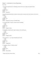
Figure 11.1
Venn Diagram for Mutually Exclusive
Events
Copyright © 2010 Pearson Education, Inc. Publishing as
Prentice Hall

11-9


Fundamentals of Probability
Non-Mutually Exclusive Events & Joint
Probability
■ Probability that non-mutually exclusive events
A and B or both will occur expressed as:
P(A or B) = P(A) + P(B) - P(AB)
■ A joint probability, P(AB), is the probability
that two or more events that are not mutually

exclusive can occur simultaneously.

Copyright © 2010 Pearson Education, Inc. Publishing as
Prentice Hall

11-


Fundamentals of Probability
Non-Mutually Exclusive Events & Joint
Probability

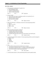
Figure 11.2
Venn Diagram for Non–Mutually Exclusive Events and
the Joint Event
Copyright © 2010 Pearson Education, Inc. Publishing as
Prentice Hall

11-


Fundamentals of Probability
Cumulative Probability Distribution
■ Can be developed by adding the probability of
an event to the sum of all previously listed
probabilities in a probability distribution.

■ Probability that a student will get a grade of C
or higher:
P(A or B or C) = P(A) + P(B) + P(C) = .10 + .20

Copyright © 2010 Pearson Education, Inc. Publishing
as
+ .50
= .80
Prentice Hall

11-


Statistical Independence and
Dependence
Independent Events
■ A succession of events that do not affect each
other are independent.
■ The probability of independent events
occurring in a succession is computed by
multiplying the probabilities of each event.
■ A conditional probability is the probability
that an event will occur given that another
event has already occurred, denoted as
P(AB). If events A and B are independent,
then:
P(AB) = P(A)  P(B) and P(AB) = P(A)
Copyright © 2010 Pearson Education, Inc. Publishing as
Prentice Hall

11-


Statistical Independence and

Dependence
Independent
– Probability
For coin tossedEvents
three consecutive
times:
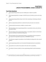
Trees

Figure
11.3

Probability of getting head on first toss, tail
on second, tail on third is .125:
P(HTT) = P(H)  P(T)  P(T) = (.5)(.5)(.5) = .125

Copyright © 2010 Pearson Education, Inc. Publishing as
Prentice Hall

11-


Statistical Independence and
Dependence
Independent Events – Bernoulli
Properties
a Bernoulli Process:
Process of
Definition
■ There are two possible outcomes for each
trial.

■ The probability of the outcome remains
constant over time.
■ The outcomes of the trials are independent.
■ The number of trials is discrete and integer.

Copyright © 2010 Pearson Education, Inc. Publishing as
Prentice Hall

11-


Statistical Independence and
Dependence
Independent Events – Binomial
A binomial probability distribution function is
Distribution
used to determine the probability of a number
of successes in n trials.
It is a discrete probability distribution since
the number of successes and trials is
discrete.
P(r)  n! prqn -r
r!(n-r)!

where: p = probability of a success
q = 1- p = probability of a failure
n = number of trials
Copyright © 2010 Pearson
Education,
Inc. Publishing

assuccesses in n trials
r
=
number
of
Prentice Hall

11-


Statistical Independence and
Dependence
Binomial Distribution Example –
Determine probability of getting exactly two
Tossed
tails inCoins
three tosses of a coin.
3! (.5)2(.5)3  2
2! (3 - 2)!
 (321) (.25)(.5)
(21)(1)
6 (.125)
2

P(2 tails) P(r 2) 

P(r 2) .375

Copyright © 2010 Pearson Education, Inc. Publishing as
Prentice Hall

11-


Statistical Independence and
Dependence
Binomial Distribution Example –
 Microchip production; sample of four
Quality
Control
items/batch,
20% of all microchips are
defective.
 What is the probability that each batch will
contain exactly two defectives?
P(r 2 defectives)  4! (.2)2(.8)2
2!(4 - 2)!
(4321)(.25)(.5)
(21)(1)
24 (.0256)
2
.1536

Copyright © 2010 Pearson Education, Inc. Publishing as
Prentice Hall

11-


Statistical Independence and

Dependence
Binomial Distribution Example –
■ Four microchips tested/batch; if two or more
Quality
Control batch is rejected.
found defective,
■ What is probability of rejecting entire batch if
batch in fact has 20% defective?
P(r 2)  4! (.2)2(.8)2  4! (.2)3(.8)1  4! (.2)4(.8)0
2!(4 - 2)!
3!(4  3)!
4!(4 - 4)!
.1536  .0256  .0016
.1808
■ Probability of less than two defectives:
P(r<2) = P(r=0) + P(r=1) = 1.0 - [P(r=2) +
P(r=3) + P(r=4)]
= 1.0 - .1808 = .8192
Copyright © 2010 Pearson Education, Inc. Publishing as
Prentice Hall

11-


Statistical Independence and
Dependence
Dependent Events (1 of 2)

Copyright © 2010 Pearson Education, Inc. Publishing as
Prentice Hall

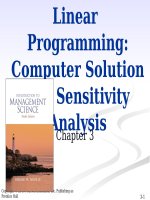
Figure 11.4
Dependent
Events

11-


Statistical Independence and
Dependence
Dependent Events (2 of 2)

■ If the occurrence of one event affects the
probability of the occurrence of another
event, the events are dependent.
■ Coin toss to select bucket, draw for blue ball.
■ If tail occurs, 1/6 chance of drawing blue ball
from bucket 2; if head results, no possibility
of drawing blue ball from bucket 1.
■ Probability of event “drawing a blue ball”
dependent on event “flipping a coin.”

Copyright © 2010 Pearson Education, Inc. Publishing as
Prentice Hall

11-


Statistical Independence and
Dependence

Dependent
Events
– Unconditional
Unconditional:
P(H) = .5;
P(T) = .5, must sum to
one.
Probabilities

Figure 11.5
Another Set of Dependent
Copyright © 2010 Pearson Education, Inc. Publishing as
Events
Prentice Hall

11-


Statistical Independence and
Dependence
DependentP(RH)
Events
– P(WH)
Conditional
Conditional:
=.33,
= .67, P(RT) = .
83, P(WT) = .17
Probabilities

Figure 11.6
Probability tree for
dependent events

Copyright © 2010 Pearson Education, Inc. Publishing as
Prentice Hall

11-


Statistical Independence and
Dependence
Math Formulation of Conditional
 Given two dependent events A and B:
Probabilities
P(AB) = P(AB)/P(B)

 With data from previous example:
P(RH) = P(RH)  P(H) = (.33)(.5) = .165
P(WH) = P(WH)  P(H) = (.67)(.5) = .335
P(RT) = P(RT)  P(T) = (.83)(.5) = .415
P(WT) = P(WT)  P(T) = (.17)(.5) = .085

Copyright © 2010 Pearson Education, Inc. Publishing as
Prentice Hall

11-


Statistical Independence and

Dependence
Summary of Example Problem
Probabilities

Figure 11.7
Copyright © 2010 Pearson Education, Inc. Publishing as
Prentice Hall

11-