Introduction to management science 10e by bernard taylor chapter 12

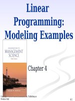
Queuing Analysis

Chapter 13

Copyright © 2010 Pearson Education, Inc. Publishing as
Prentice Hall

13-1


Chapter Topics
■ Elements of Waiting Line Analysis
■ The Single-Server Waiting Line System
■ Undefined and Constant Service Times
■ Finite Queue Length
■ Finite Calling Problem
■ The Multiple-Server Waiting Line
■ Additional Types of Queuing Systems

Copyright © 2010 Pearson Education, Inc. Publishing as
Prentice Hall

13-2


Overview
 Significant amount of time spent in waiting lines by
people, products, etc.
 Providing quick service is an important aspect of
quality customer service.
 The basis of waiting line analysis is the trade-off

between the cost of improving service and the costs
associated with making customers wait.
 Queuing analysis is a probabilistic form of analysis.
 The results are referred to as operating
characteristics.
 Results are used by managers of queuing operations
to make decisions.
Copyright © 2010 Pearson Education, Inc. Publishing as
Prentice Hall

13-3


Elements of Waiting Line
Analysis (1 of 2)
 Waiting lines form because people or
things arrive at a service faster than
they can be served.
 Most operations have sufficient server
capacity to handle customers in the long
run.
 Customers however, do not arrive at a
constant rate nor are they served in an
equal amount of time.
Copyright © 2010 Pearson Education, Inc. Publishing as
Prentice Hall

13-4

Elements of Waiting Line
Analysis (2 of 2)
 Waiting lines are continually increasing and
decreasing in length and approach an
average rate of customer arrivals and an
average service time, in the long run.
 Decisions concerning the management of
waiting lines are based on these averages
for customer arrivals and service times.
 They are used in formulas to compute
operating characteristics of the system
Copyright © 2010 Pearson Education, Inc. Publishing as
Prentice Hall

13-5


The Single-Server Waiting Line System
(1 of 2)
 Components of a waiting line system include
arrivals (customers), servers, (cash
register/operator), customers in line form a waiting
line.
 Factors to consider in analysis:


The queue discipline.



The nature of the calling population



The arrival rate



The service rate.

Copyright © 2010 Pearson Education, Inc. Publishing as
Prentice Hall

13-6


The Single-Server Waiting Line
System (2 of 2)

Figure
13.1
Copyright © 2010 Pearson Education, Inc. Publishing as
Prentice Hall

13-7


Single-Server Waiting Line System
Component Definitions


Queue Discipline: The order in which waiting
customers are served.



Calling Population: The source of customers
(infinite or finite).



Arrival Rate: The frequency at which customers
arrive at a waiting line according to a probability
distribution (frequently described by a Poisson
distribution).



Service Rate: The average number of customers
that can be served during a time period (often
described by the negative exponential distribution).

Copyright © 2010 Pearson Education, Inc. Publishing as
Prentice Hall

13-8


Single-Server Waiting Line System
Single-Server Model





Assumptions of the basic single-server model:


An infinite calling population



A first-come, first-served queue discipline



Poisson arrival rate



Exponential service times

Symbols:
λ = the arrival rate (average number of arrivals/time
period)
µ = the service rate (average number served/time
period)



Customers must be served faster than they arrive (λ

Copyright © 2010 Pearson Education, Inc. Publishing as
Prentice Hall

13-9


Single-Server Waiting Line System
Basic Single-Server Queuing
Formulas (1 of 2)
Probability that no customers are in the
queuing system:


÷
P0 =  1− λ
÷
µ



Probability that n customers
are in the system:
n
n



 


÷ ×P =  λ ÷  1− λ ÷
Pn =  λ
µ÷ 0 µ÷  µ÷












L= λ
µ −λ
Average number of customers in system:

2
λ
Lq = 
µ  µ − λ ÷
Average number of customer in the waiting line:13-

Copyright © 2010 Pearson Education, Inc. Publishing as
Prentice Hall


Single-Server Waiting Line System

Basic Single-Server Queuing
Formulas (2 of 2)
Average time customer spends waiting and
being served:
W= 1 =L
µ −λ λ

Average time customer
waiting in the
λ
Wq = spends
µ  µ − λ ÷
queue:

U=λ
µ

Probability that server is busy (utilization
I = 1− U = 1− λ
factor):
µ
Probability that server is idle:

Copyright © 2010 Pearson Education, Inc. Publishing as
Prentice Hall

13-


Single-Server Waiting Line System

Operating Characteristics: Fast Shop
Market
(1 of 2) per hour arrive at checkout
λ = 24 customers
counter

µ = 30λ ÷customers per hour can be checked out
P0 =  1− µ ÷= (1 - 24/30)




= .20 probability of no customers in the system

L = λ = 24/(30 - 24) = 4 customers on the avg in the system
µ −λ
2
λ
Lq = 
µ  µ − λ ÷
= (24)2 /[30(30 -24)] = 3.2 customers on the avg in the waiting line
Copyright © 2010 Pearson Education, Inc. Publishing as
Prentice Hall

13-


Single-Server Waiting Line System
Operating Characteristics for Fast Shop
Market

(2
of 2)
1
L
W=

= = 1/[30 -24]
µ −λ λ
= 0.167 hour (10 min) avg time in the system per customer

λ = 24/[30(30 -24)]
µ  µ − λ ÷
= 0.133 hour (8 min) avg time in the waiting line

Wq =

U=λ
µ = 24/30

= .80 probability server busy, .20 probability server will be idle

Copyright © 2010 Pearson Education, Inc. Publishing as
Prentice Hall

13-


Single-Server Waiting Line System
Steady-State Operating
Characteristics

Because of steady-state nature of operating
characteristics:


Utilization factor, U, must be less than one:
U < 1, or λ / µ < 1 and λ < µ.



The ratio of the arrival rate to the service
rate must be
less than one or, the
service rate must be greater than
the
arrival rate.

The server must be able to serve
customers faster than
the arrival rate
Copyright © 2010
Pearson
Education,
Inc.
Publishing
aswaiting line will grow
in
the
long
run,
or

Prentice Hall


13-


Single-Server Waiting Line System
Effect of Operating Characteristics
(1 of
6) wishes to test several alternatives for
Manager
reducing customer waiting time:
1.

2.

Addition of another employee to pack up
purchases
Addition of another checkout counter.

Alternative 1: Addition of an employee
(raises service rate from µ = 30 to µ = 40 customers
per hour).


Cost $150 per week, avoids loss of $75 per
week for each minute of reduced customer
waiting time.

System operating characteristics with new

Copyright © 2010
Pearson Education, Inc. Publishing as
parameters:
Prentice Hall


13-


Single-Server Waiting Line System
Effect of Operating Characteristics
 System
(2 of
6) operating characteristics with new
parameters

(continued):

Lq = 0.90 customer on the average in the waiting
line
W = 0.063 hour average time in the system per
customer
Wq = 0.038 hour average time in the waiting line
per customer
U = .60 probability that server is busy and
customer must wait
I = .40 probability that server is available
Average customer waiting time reduced from 8 to 2.25
minutes worth $431.25 per week.
Copyright © 2010 Pearson Education, Inc. Publishing as

Prentice Hall

13-


Single-Server Waiting Line System
Effect of Operating Characteristics
(3Alternative
of 6) 2: Addition of a new checkout counter ($6,000
plus $200 per week for additional cashier).





λ = 24/2 = 12 customers per hour per checkout
counter
µ = 30 customers per hour at each counter
System operating characteristics with new
parameters:
Po = .60 probability of no customers in the system
L = 0.67 customer in the queuing system
Lq = 0.27 customer in the waiting line
W = 0.055 hour per customer in the system
Wq = 0.022 hour per customer in the waiting line
U = .40 probability that a customer must wait

Copyright © 2010 Pearson Education, Inc. Publishing as
Prentice Hall

13-


Single-Server Waiting Line System
Effect of Operating Characteristics
(4 of 6)
Savings from reduced waiting time worth:
$500 per week - $200 = $300 net savings
per week.
After $6,000 recovered, alternative 2 would
provide:
$300 -281.25 = $18.75 more savings per
week.

Copyright © 2010 Pearson Education, Inc. Publishing as
Prentice Hall

13-


Single-Server Waiting Line System
Effect of Operating Characteristics
(5 of 6)

Table 13.1
Operating Characteristics for Each Alternative
Copyright © 2010 Pearson Education, Inc. Publishing as
System
Prentice Hall

13-


Single-Server Waiting Line System
Effect of Operating Characteristics
(6 of 6)

Figure 13.2

Cost Trade-Offs for Service

Copyright © 2010 Pearson Education, Inc. Publishing as
Prentice Hall

13-


Single-Server Waiting Line System
Solution with Excel and Excel QM (1
of 2)

Copyright © 2010 Pearson Education, Inc. Publishing as
Prentice Hall

Exhibit 13.1

13-


Single-Server Waiting Line System

Solution with Excel and Excel QM (2
of 2)

Copyright © 2010 Pearson Education, Inc. Publishing as
Prentice Hall

Exhibit 13.2

13-


Single-Server Waiting Line System
Solution with QM for Windows

Copyright © 2010 Pearson Education, Inc. Publishing as
Prentice Hall

Exhibit 13.3

13-


Single-Server Waiting Line System
Undefined and Constant Service
Times
 Constant, rather than exponentially
distributed service times, occur with
machinery and automated equipment.
 Constant service times are a special case of
the single-server model with undefined

service times.
Lq
λ
P
=
1
−
Wq =
 Queuing formulas:
0
µ
λ
2
λ 2σ 2 +  λ / µ ÷
Lq =
2 1− λ / µ ÷

1
W =Wq + µ

L = Lq + λ
µ

U=λ
µ

Copyright © 2010 Pearson Education, Inc. Publishing as
Prentice Hall

13-

Single-Server Waiting Line System
Undefined Service Times Example (1
of 2)
Data: Single fax machine; arrival rate of 20
users per hour, Poisson distributed; undefined
service time with mean of 2 minutes,
standard deviation of 4 minutes.
 Operating characteristics:
20 = .33 probability that machine not in use
P0 = 1− λ
=
1
−
µ
30
2  2 
2 
2




2
2
λ σ +  λ / µ ÷  20 ÷  1/15 ÷ +  20/ 30 ÷
Lq =
=



2 1− λ / µ ÷
2 1− 20/ 30 ÷
= 3.33 employees waiting in line
L = Lq + λ
µ = 3.33 + (20/ 30)

= 4.0 employees in line and using the machine

Copyright © 2010 Pearson Education, Inc. Publishing as
Prentice Hall

13-