Introduction to management science 10e by bernard taylor chapter 14

Simulation

Chapter 14

Copyright © 2010 Pearson Education, Inc. Publishing as
Prentice Hall

14-1


Chapter Topics
■The Monte Carlo Process
■Computer Simulation with Excel
Spreadsheets
■Simulation of a Queuing System
■Continuous Probability Distributions
■Statistical Analysis of Simulation Results
■Crystal Ball
■Verification of the Simulation Model
■Areas of Simulation Application
Copyright © 2010 Pearson Education, Inc. Publishing as
Prentice Hall

14-2


Overview
■ Analogue simulation replaces a physical system
with an analogous physical system that is easier to
manipulate.
■ In computer mathematical simulation a system

is replaced with a mathematical model that is
analyzed with the computer.
■ Simulation offers a means of analyzing very
complex systems that cannot be analyzed using
the other management science techniques in the
text.
Copyright © 2010 Pearson Education, Inc. Publishing as
Prentice Hall

14-3


Monte Carlo Process
■ A large proportion of the applications of simulations
are for probabilistic models.
■ The Monte Carlo technique is defined as a
technique for selecting numbers randomly from a
probability distribution for use in a trial (computer
run) of a simulation model.
■ The basic principle behind the process is the same
as in the operation of gambling devices in casinos
(such as those in Monte Carlo, Monaco).
Copyright © 2010 Pearson Education, Inc. Publishing as
Prentice Hall

14-4


Monte Carlo Process
Use of Random Numbers (1 of 10)



In the Monte Carlo process, values for a random
variable are generated by sampling from a
probability distribution.



Example: ComputerWorld demand data for laptops
selling for $4,300 over a period of 100 weeks.

Table 14.1 Probability Distribution of Demand
for Laptop PC’s

Copyright © 2010 Pearson Education, Inc. Publishing as
Prentice Hall

14-5


Monte Carlo Process
Use of Random Numbers (2 of 10)


The purpose of the Monte Carlo process is
to generate the random variable,
demand, by sampling from the probability
distribution P(x).



The partitioned roulette wheel replicates the
probability distribution for demand if the
values of demand occur in a random
manner.



The segment at which the wheel stops

Copyright © 2010 Pearson Education, Inc. Publishing as
Prentice Hall

14-6


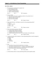
Monte Carlo Process
Use of Random Numbers (3 of 10)

Figure 14.1 A Roulette Wheel
for Demand

Copyright © 2010 Pearson Education, Inc. Publishing as
Prentice Hall

14-7


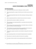
Monte Carlo Process
Use of Random Numbers (4 of 10)

When the wheel is spun, the actual demand for PCs is
determined by a number at rim of the wheel.

Figure 14.2
umbered Roulette Wheel
Copyright © 2010 Pearson Education, Inc. Publishing as
Prentice Hall

14-8


Monte Carlo Process
Use of Random Numbers (5 of 10)

Table 14.2 Generating Demand from
Random Numbers

Copyright © 2010 Pearson Education, Inc. Publishing as
Prentice Hall

14-9


Monte Carlo Process
Use of Random Numbers (6 of 10)
Select number from a random number table:

Copyright © 2010 Pearson Education, Inc. Publishing as
Prentice Hall

Table 14.3
Numbers

Delightfully Random
14-


Monte Carlo Process
Use of Random Numbers (7 of 10)


Repeating selection of random numbers
simulates demand for a period of time.



Estimated average demand = 31/15 = 2.07
laptop PCs per week.



Estimated average revenue = $133,300/15
= $8,886.67.

Copyright © 2010 Pearson Education, Inc. Publishing as
Prentice Hall

14-

Monte Carlo Process
Use of Random Numbers (8 of 10)

Copyright © 2010 Pearson Education, Inc. Publishing as
Prentice Hall

Table 14.4

14-


Monte Carlo Process
Use of Random Numbers (9 of 10)
Average demand could have been calculated
analytically:
n
E( x) = ∑ P( xi) xi
i=1

where:
xi = demand value i
P( xi) = probability of demand
n = the number of different demand values
therefore:
E( x) = (.20)(0) + (.40)(1) + (.20)(2) + (.10)(3) + (.10)(4)
= 1.5 PC's per week
Copyright © 2010 Pearson Education, Inc. Publishing as
Prentice Hall

14-

Monte Carlo Process
Use of Random Numbers (10 of 10)


The more periods simulated, the more accurate
the results.



Simulation results will not equal analytical results
unless enough trials have been conducted to reach
steady state.



Often difficult to validate results of simulation that true steady state has been reached and that
simulation model truly replicates reality.



When analytical analysis is not possible, there is no
14analytical standard of comparison thus making

Copyright © 2010 Pearson Education, Inc. Publishing as
Prentice Hall


Computer Simulation with Excel

Spreadsheets
Generating Random Numbers (1 of
2) As simulation models get more complex they
become impossible to perform manually.



In simulation modeling, random numbers are
generated by a mathematical process instead
of a physical process (such as wheel spinning).



Random numbers are typically generated on the
computer using a numerical technique and thus are
not true random numbers but pseudorandom
numbers.

Copyright © 2010 Pearson Education, Inc. Publishing as
Prentice Hall

14-


Computer Simulation with Excel
Spreadsheets
Generating Random Numbers (2 of
2)
Artificially created random numbers must have
the following characteristics:

1.

The random numbers must be
uniformly distributed.

2.

The numerical technique for generating
the numbers must be efficient.

3.

The sequence of random numbers should
reflect no pattern.

Copyright © 2010 Pearson Education, Inc. Publishing as
Prentice Hall

14-


Simulation with Excel Spreadsheets
(1 of 3)

Copyright © 2010 Pearson Education, Inc. Publishing as
Prentice Hall

Exhibit 14.1
14-

Simulation with Excel Spreadsheets
(2 of 3)

Copyright © 2010 Pearson Education, Inc. Publishing as
Prentice Hall

Exhibit 14.2

14-


Simulation with Excel Spreadsheets
(3 of 3)

Copyright © 2010 Pearson Education, Inc. Publishing as
Prentice Hall

Exhibit 14.3

14-


Computer Simulation with Excel
Spreadsheets
Decision
Making example;
with Simulation
(1 laptop
Revised ComputerWorld

order size of one
each
of
2)week.

Exhibit 14.4

Copyright © 2010 Pearson Education, Inc. Publishing as
Prentice Hall

14-


Computer Simulation with Excel
Spreadsheets
Decision
with Simulation
Order sizeMaking
of two laptops
each week. (2
of 2)

Exhibit 14.5

Copyright © 2010 Pearson Education, Inc. Publishing as
Prentice Hall

14-

Simulation of a Queuing System
Burlingham Mills Example (1 of 3)

Table 14.5 Distribution of
Arrival Intervals

Table 14.6 Distribution of

Copyright © 2010 Pearson Education, Inc. Publishing as
Prentice Hall

14-


Simulation of a Queuing System
Burlingham Mills Example (2 of 3)

Average waiting time = 12.5days/10 batches
= 1.25 days per batch
Average time in the system = 24.5 days/10
batches
Copyright
© 2010 Pearson Education, Inc. Publishing as
Prentice Hall
= 2.45 days per batch

14-


Simulation of a Queuing System

Burlingham Mills Example (3 of 3)
Caveats:
■

Results may be viewed with skepticism.

■

Ten trials do not ensure steady-state
results.

■

Starting conditions can affect
simulation results.

■

If no batches are in the system at start,
simulation must run until it replicates
normal operating system.

If system starts with items already in the
Copyright © 2010 Pearson Education, Inc. Publishing as
simulation must begin with
Prentice Hall system,
14■


Computer Simulation with Excel

Burlingham Mills Example

Exhibit 14.6
Copyright © 2010 Pearson Education, Inc. Publishing as
Prentice Hall

14-