Introduction to operations and supply chain management 3e bozarth chapter 06

Managing Capacity
Chapter 6


Chapter Objectives
Be able to:
 Explain what capacity is, how firms measure capacity, and the
difference between theoretical and rated capacity.
 Describe the pros and cons associated with three different
capacity strategies: lead, lag, and match.
 Apply a wide variety of analytical tools to capacity decisions,
including expected value and break-even analysis, decision
trees, learning curves, the Theory of Constraints, waiting line
theory, and Little’s Law.

Copyright © 2013 Pearson Education, Inc. publishing as Prentice Hall

6-2


Definitions
 Capacity – The capability of a worker, a machine, a
workcenter, a plant, or an organization to produce
output in a time period.
 Capacity decisions
–
© 2010 APICS Dictionary
 How is it measured?
 Which factors affect capacity?
 The impact of the supply chain on the organization’s
effective capacity.

Copyright © 2013 Pearson Education, Inc. publishing as Prentice Hall

6-3


Measures of Capacity
 Theoretical capacity – The maximum output
capability, allowing for no adjustments for
preventive maintenance, unplanned downtime, or
the like.
 Rated capacity – The long-term, expected output
capability of a resource or system.
© 2010 APICS Dictionary

Copyright © 2013 Pearson Education, Inc. publishing as Prentice Hall

6-4


Examples of Capacity

Table 6.1

Copyright © 2013 Pearson Education, Inc. publishing as Prentice Hall

6-5


Indifference Point Examples

Capacity for a PC Assembly Plant
(800 units per line per shift)×(# of lines)×(# of shifts)
Controllable Factors

Uncontrollable Factors

1 or 2 shifts?
2 or 3 lines? Employee
training?

Supplier problems?
98% or 100% good?
Late or on time?

Copyright © 2013 Pearson Education, Inc. publishing as Prentice Hall

6-6


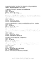
Three Common
Capacity Strategies
 Lead capacity strategy – A capacity strategy in which
capacity is added in anticipation of demand.
 Lag capacity strategy – A capacity strategy in which
capacity is added only after demand has
materialized.
 Match capacity strategy – A capacity strategy that
strikes a balance between the lead and lag capacity
strategies by avoiding period of high under or
overutilization.

Copyright © 2013 Pearson Education, Inc. publishing as Prentice Hall

6-7


Comparing Strategies

Figure 6.1

Copyright © 2013 Pearson Education, Inc. publishing as Prentice Hall

6-8


Evaluating Capacity Alternatives






Cost Comparison
Expected Value
Decision Trees
Break-Even Analysis
Learning Curves

Copyright © 2013 Pearson Education, Inc. publishing as Prentice Hall

6-9

Cost Comparison
 Fixed costs – The expenses an organization incurs
regardless of the level of business activity.
 Variable costs – Expenses directly tied to the level of
business activity.

Copyright © 2013 Pearson Education, Inc. publishing as Prentice Hall

6 - 10


Cost Comparison
TC = FC + VC * X
TC = Total Cost
FC = Fixed Cost
VC = Variable cost per unit of business activity
X = amount of business activity

Copyright © 2013 Pearson Education, Inc. publishing as Prentice Hall

6 - 11


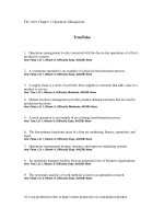
Cost Comparison - Example 6.1

Table 6.2

Figure 6.2

Copyright © 2013 Pearson Education, Inc. publishing as Prentice Hall

6 - 12


Cost Comparison - Example 6.1
Total cost of common carrier option = Total cost of contract carrier option
$0 + $750X = $5,000 + $300X
X = 11.11 or 11 shipments

Find the indifference point – the output level at which
the two alternatives generate equal costs.
Total cost of contract carrier option = Total cost of leasing
$5,000 + $300X = $21,000 + $50X
X = 64 shipments
Copyright © 2013 Pearson Education, Inc. publishing as Prentice Hall

6 - 13


Expected Value
 Expected value – A calculation that summarizes the
expected costs, revenues, or profits of a capacity
alternative, based on several demand levels with
different probabilities.

Copyright © 2013 Pearson Education, Inc. publishing as Prentice Hall

6 - 14

Expected Value – Example 6.2

Copyright © 2013 Pearson Education, Inc. publishing as Prentice Hall

6 - 15


Expected Value – Example 6.2
C(low demand) = $5,000 + $300(30) = $14,000
C(medium demand) = $5,000 + $300(50) = $20,000
C(high demand) = $5,000 + $300(80) = $29,000
EVContract = (14,000 * 25%) + ($20,000 * 60%) + ($29,000 * 15%)
= $19,850
EVCommon = (22,500 * 25%) + ($37,500 * 60%) + ($60,000 * 15%)
= $37,125
EVLease = (22,500 * 25%) + ($23,500 * 60%) + ($25,000 * 15%)
= $23,475
Copyright © 2013 Pearson Education, Inc. publishing as Prentice Hall

6 - 16


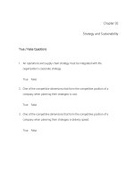
Decision Trees
 Decision tree – A visual tool that decision makers
use to evaluate capacity decisions to enable users to
see the interrelationships between decisions and
possible outcomes.

Copyright © 2013 Pearson Education, Inc. publishing as Prentice Hall

6 - 17


Decision Tree Rules
 Draw the tree from left to right starting with a
decision point or an outcome point and develop
branches from there.
 Represent decision points with squares.
 Represent outcome points with circles.
 For expected value problems, calculate the financial
results for each of the smaller branches and move
backward by calculating weighted averages for the
branches based on their probabilities.
Copyright © 2013 Pearson Education, Inc. publishing as Prentice Hall

6 - 18


Decision Trees – Example 6.3
Original Expected
Value Example

Figure 6.4
Copyright © 2013 Pearson Education, Inc. publishing as Prentice Hall

6 - 19


Break-Even Analysis

 Break-even point – The volume level for a business
at which total revenues cover total costs.

Where:

BEP = break-even point
FC = fixed costs
VC = variable cost per unit of business activity
R = revenue per unit of business activity

Copyright © 2013 Pearson Education, Inc. publishing as Prentice Hall

6 - 20


Break-Even Analysis – Example 6.4
Suppose the firm makes $1,000 profit on each shipment
before transportation costs are considered. What is the
break-even point for each shipping option?

Contracting: BEP = $5,000 / $700 = 7.1 or 8 shipments
Common: BEP = $0 / $250 = 0 shipments
Leasing: BEP = $21,000 / $950 = 22.1 or 23 shipments

Copyright © 2013 Pearson Education, Inc. publishing as Prentice Hall

6 - 21


Learning Curves

 Learning curve theory – A theory that suggests that
productivity levels can improve at a predictable rate
as people and even systems “learn” to do tasks
more efficiently.
For every doubling of cumulative output, there
is a set percentage reduction in the amount
of inputs required.

Copyright © 2013 Pearson Education, Inc. publishing as Prentice Hall

6 - 22


Learning Curves

Copyright © 2013 Pearson Education, Inc. publishing as Prentice Hall

6 - 23


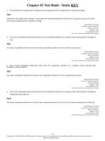
Learning Curve – Example 6.5

What is the learning percentage?
4/5 = 80% or .80

Copyright © 2013 Pearson Education, Inc. publishing as Prentice Hall

6 - 24

Learning Curve – Example 6.5
How long will it take to answer the 25th call?

Figure 6.6
Copyright © 2013 Pearson Education, Inc. publishing as Prentice Hall

6 - 25