Introduction to operations and supply chain management 3e bozarth chapter 09

Forecasting
Chapter 9


Chapter Objectives
Be able to:

Discuss the importance of forecasting and identify the
most appropriate type of forecasting approach, given
different forecasting situations.
Apply a variety of time series forecasting models,
including moving average, exponential smoothing, and
linear regression models.
Develop causal forecasting models using linear
regression and multiple regression.
Calculate measures of forecasting accuracy and
interpret the results.
Copyright © 2013 Pearson Education, Inc. publishing as Prentice Hall

9-2


Forecasting
 Forecast – An estimate of the future level of
some variable.
 Why Forecast?

 Assess long-term capacity needs
 Develop budgets, hiring plans, etc.
 Plan production or order materials

Copyright © 2013 Pearson Education, Inc. publishing as Prentice Hall

9-3


Types of Forecasts
 Demand
 Firm-level
 Market-level

 Supply
 Number of current producers and suppliers
 Projected aggregate supply levels
 Technological and political trends

 Price
 Cost of supplies and services
 Market price for firm’s product or service
Copyright © 2013 Pearson Education, Inc. publishing as Prentice Hall

9-4


Laws of Forecasting
 Forecasts are almost always wrong by some amount
(but they are still useful).
 Forecasts for the near term tend to be more
accurate.
 Forecasts for groups of products or services tend to
be more accurate.

 Forecasts are no substitute for calculated values.
Copyright © 2013 Pearson Education, Inc. publishing as Prentice Hall

9-5


Forecasting Methods
 Qualitative forecasting techniques – Forecasting
techniques based on intuition or informed opinion.
 Used when data are scarce, not available, or
irrelevant.
 Quantitative forecasting models – Forecasting
models that use measurable, historical data to
generate forecasts.
 Time series and causal models
Copyright © 2013 Pearson Education, Inc. publishing as Prentice Hall

9-6


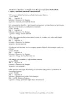
Selecting a Forecasting Method

Figure 9.2
Copyright © 2013 Pearson Education, Inc. publishing as Prentice Hall

9-7


Qualitative Forecasting Methods
 Market surveys

 Build-up forecasts
 Life-cycle analogy method
 Panel consensus forecasting
 Delphi method

Copyright © 2013 Pearson Education, Inc. publishing as Prentice Hall

9-8


Quantitative Forecasting Methods
 Time series forecasting models – Models that
use a series of observations in chronological
order to develop forecasts.
 Causal forecasting models – Models in which
forecasts are modeled as a function of
something other than time.

Copyright © 2013 Pearson Education, Inc. publishing as Prentice Hall

9-9


Demand movement
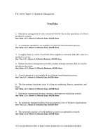
 Randomness – Unpredictable movement from one
time period to the next.
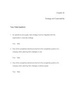
 Trend – Long-term movement up or down in a time
series.
 Seasonality – A repeated pattern of spikes or drops
in a time series associated with certain times of the

year.
Copyright © 2013 Pearson Education, Inc. publishing as Prentice Hall

9 - 10


Time series with randomness

Figure 9.3

Copyright © 2013 Pearson Education, Inc. publishing as Prentice Hall

9 - 11


Time series with
Trend and Seasonality

Figure 9.4

Copyright © 2013 Pearson Education, Inc. publishing as Prentice Hall

9 - 12


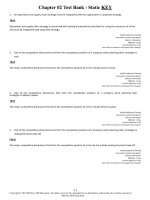
Last Period Model
 Last Period Model - The simplest time series
model that uses demand for the current
period as a forecast for the next period.

Ft+1 = Dt
where Ft+1= forecast for the next period, t+1
and Dt = demand for the current period, t

Copyright © 2013 Pearson Education, Inc. publishing as Prentice Hall

9 - 13


Last Period Model

Table 9.3

Figure 9.5
Copyright © 2013 Pearson Education, Inc. publishing as Prentice Hall

9 - 14


Moving Average Model
 Moving Average Model – A time series
forecasting model that derives a forecast by
taking an average of recent demand value.
n

D

t 1 i

Ft 1  i 1

n

Copyright © 2013 Pearson Education, Inc. publishing as Prentice Hall

9 - 15


Moving Average Model
Period
1
2
3
4
5
6
7
8

Demand
12
15
11
9
10
8
14
12

n

Ft 1 

 Dt 1 i

i 1

n

3-period moving average
forecast for Period 8:
=
=

(14 + 8 + 10) / 3
10.67

Copyright © 2013 Pearson Education, Inc. publishing as Prentice Hall

9 - 16


Weighted Moving Average Model
 Weighted Moving Average Model – A form of
the moving average model that allows the
actual weights applied to past observations
to differ.

Copyright © 2013 Pearson Education, Inc. publishing as Prentice Hall

9 - 17


Weighted Moving Average Model
Period
1
2
3
4
5
6
7
8

Demand
12
15
11
9
10
8
14
12

3-period weighted moving
average forecast for Period 8=

[(0.5  14) + (0.3  8) + (0.2  10)] / 1
=
11.4

Copyright © 2013 Pearson Education, Inc. publishing as Prentice Hall

9 - 18


Exponential Smoothing Model
 Exponential Smoothing Model – A form of the
moving average model in which the forecast for the
next period is calculated as the weighted average of
the current period’s actual value and forecast.

Copyright © 2013 Pearson Education, Inc. publishing as Prentice Hall

9 - 19


Exponential Smoothing Model
 = .3
Period Demand
Forecast
1
50
40
 
 
 
2
46
.3 * 50 + (1-.3) * 40 = 43
 

 
 
3
52
.3 * 46 + (1-.3) * 43 = 43.9
 
 
 
4
48
.3 * 52 + (1-.3) * 43.9 = 46.33
 
 
 
5
47
.3 * 48 + (1-.3) * 46.33 = 46.83
 
 
 
6
 
.3 * 47 + (1-.3) * 46.83 = 46.88

Copyright © 2013 Pearson Education, Inc. publishing as Prentice Hall

9 - 20


Adjusted Exponential Smoothing

 Adjusted Exponential Smoothing Model – An expanded
version of the exponential smoothing model that includes a
trend adjustment factor.

AFt+1 = Ft+1 +Tt+1
where AFt+1 = adjusted forecast for the next period
Ft+1 = unadjusted forecast for the next period = Dt + (1 – ) Ft
Tt+1 = trend factor for the next period = (Ft+1 – Ft) + (1 – )Tt
Tt = trend factor for the current period
smoothing constant for the trend adjustment factor
Copyright © 2013 Pearson Education, Inc. publishing as Prentice Hall

9 - 21


Linear Regression

Copyright © 2013 Pearson Education, Inc. publishing as Prentice Hall

9 - 22


Linear Regression
 How to calculate the a and b

Copyright © 2013 Pearson Education, Inc. publishing as Prentice Hall

9 - 23

Linear Regression – Example 9.3

Copyright © 2013 Pearson Education, Inc. publishing as Prentice Hall

9 - 24


Linear Regression – Example 9.3

Copyright © 2013 Pearson Education, Inc. publishing as Prentice Hall

9 - 25