Solution manual auditing and services 2e by louwers MODE

Module E - Overview of Sampling

MODULE E
Overview of Sampling
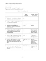
LEARNING OBJECTIVES
Review
Checkpoints

Exercises, Problems,
and Simulations

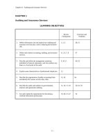
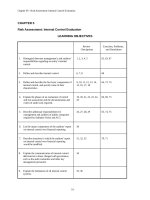
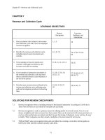
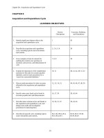
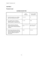
1.

Understand the basic principles of sampling,
including the differences between statistical and
nonstatistical sampling and sampling and
nonsampling risk.

1, 2, 3, 4, 5, 6

51, 52, 53, 54, 55
(parts a – c), 56, 63
(parts a – c), 66, 67,
71 (parts a – e)

2.

Understand the basic steps and procedures used
in conducting a sampling plan.

7, 8, 9, 10, 11, 12,

13

55 (part d), 57, 58,
59, 60, 61, 62, 63
(parts d – g), 64, 65,
68, 70

3.

Identify the two situations in which sampling is
used in an audit examination.

14, 15, 16, 17, 18,
19, 20, 21

71

4.

Understand how the basic steps and procedures
used in a sampling plan apply to an audit
examination.

22, 23, 24

69, 72, 73, 74

SOLUTIONS FOR REVIEW CHECKPOINTS
E.1

Sampling can be used by the auditor during the study and evaluation of a client’s internal control
and the substantive procedures.

E.2

Sampling risk is the possibility that the decision made based on the sample differs from the
decision that would have been made if the entire population had been examined, a sampling error.
Sampling error arises when the sample drawn from the population does not appropriately represent
that population.

E.3

Nonsampling risk represents the probability that an incorrect conclusion is reached because of
reasons unrelated to the nature of the sample, a nonsampling error. Nonsampling error arises
because of errors in judgment or execution of the sampling plan.

E.4

Sampling risk is controlled by the auditor by (1) determining an appropriate sample size and (2)
evaluating sample results to consider the possibility that the sample does not appropriately
represent the population.

MODE-1


Module E - Overview of Sampling

E.5

Statistical sampling plans apply the laws of probability to select sample items for examination and

evaluate sample results. Statistical sampling plans differ from nonstatistical sampling plans in
terms of the methods used to determine the appropriate sample size and evaluate the sample
results. In a statistical sampling plan, these methods control exposure to sampling risk, whereas
they do not do so in a nonstatistical sampling plan.

E.6

Either statistical sampling or nonstatistical sampling can be used under generally accepted auditing
standards. Nonstatistical sampling should not be used solely to reduce sample size.

E.7

1.
2.
3.
4.
5.
6.
7.

E.8

It is important to carefully define the population of interest, since the results of the entire sampling
application will be based on the population from which the sample is drawn.

E.9

Sampling risk has an inverse relationship with sample size; that is, as a lower level of sampling
risk is necessary, the individual needs to select a larger sample (and vice versa).

E.10

Four methods commonly used to select sample items are (1) unrestricted random selection, (2)
systematic random selection, (3) haphazard selection, and (4) block selection.

Determine the objective of sampling
Define the characteristic of interest
Define the population
Determine the sample size
Select sample items
Measure sample items
Evaluate the sample results

When using unrestricted random selection, a series of random numbers is identified and the
random numbers are matched to numbered items in the corresponding population.
When using systematic random selection, a random starting point is selected within the
population. A fixed number of items are bypassed and the corresponding item in the population is
selected. This process is continued until a number of items equal to the appropriate sample size is
selected.
Haphazard selection identifies sample items in a nonsystematic manner, with no deliberate effort
to match random numbers to sample items.
E.11

E.12

Block selection identifies a series of contiguous (adjacent) units for selection.
Unrestricted random selection or systematic random selection are used with statistical sampling
because these methods (1) provide a reasonable likelihood of selecting a representative sample, (2)
allow the probability of selecting sample items to be determined, and (3) allow the sample
selection process to be replicated.

The precision (or allowance for sampling risk) is the numeric distance from the estimated
population value in which the true (but unknown) population value may lie with a given
probability.
Reliability (or confidence) is the likelihood of achieving a given level of precision.
The precision interval is a range around the sample estimate that has a likelihood equal to
reliability (or 100 percent minus the sampling risk) of including the true population value.

MODE-2


Module E - Overview of Sampling
E.13

The following are the basic steps in evaluating sample results:
1.
2.
3.
4.

Select and measure sample items to determine the sample estimate.
Based on the acceptable sampling risk, determine the reliability and related precision.
Form the precision interval by adding and subtracting the precision from the sample
estimate.
Determine whether the hypothesized (or acceptable) value falls within the precision
interval.

E.14

Attribute sampling is used to determine the extent to which a particular characteristic (or attribute)
exists within a population. In an audit examination, attribute sampling is used in the study and

evaluation of internal control and subsequent assessment of control risk.

E.15

The tolerable deviation rate is the maximum rate of deviations from a control that an auditor will
permit without reducing the planned reliance on internal control. The auditor will compare an
“adjusted” sample deviation rate (upper limit deviation rate) to the tolerable deviation rate to
determine the extent to which the auditor can rely on internal control.

E.16

The risk of assessing control risk too high (risk of underreliance) occurs when the auditor’s sample
indicates that the control is not functioning effectively when, in fact, it is doing so. When this risk
occurs, the auditor’s upper limit deviation rate exceeds the tolerable deviation rate. However,
unknown to the auditor, the true population deviation rate is less than the tolerable deviation rate.
The risk of assessing control risk too low (risk of overreliance) occurs when the auditor’s sample
indicates that the control is functioning effectively when, in fact, it is not. When this risk occurs,
the auditor’s upper limit deviation rate is less than the tolerable deviation rate. However, unknown
to the auditor, the true population deviation rate exceeds the tolerable deviation rate.
The assessing control risk too high results in an efficiency loss for the auditor, since more
extensive substantive procedures are performed than is necessary. The assessing control risk too
low exposes the auditor to an effectiveness loss, since the auditor’s substantive procedures will not
reduce audit risk to the acceptable level.

E.17

The risk of assessing control risk too low is of greater concern to the auditor, since it may
eventually result in the auditor issuing an unqualified opinion on financial statements that are
materially misstated.

E.18

Variables sampling is used to examine a population when the auditor wants to estimate the amount
(or value) of some characteristic of that population. Variables sampling is used by the auditor
when performing substantive procedures to evaluate the fairness of an account balance or class of
transactions.

E.19

Tolerable error is the amount of misstatement that the auditor is willing to allow in an account
balance or class of transactions without concluding that it is materially misstated. The auditor will
compare an “adjusted” sample misstatement (upper error limit) to the tolerable error to determine
whether the account balance is materially misstated.

E.20

The two sampling risks associated with variables sampling are the risk of incorrect acceptance and
the risk of incorrect rejection. The risk of incorrect acceptance is the likelihood that the sample
results indicate the account balance is fairly stated when, in fact, it is materially misstated. The
risk of incorrect rejection is the likelihood that the sample results indicate the account balance is
materially misstated when, in fact, it is fairly stated.

MODE-3


Module E - Overview of Sampling

Incorrect acceptance exposes the auditor to an effectiveness loss, because the auditor will make an
incorrect conclusion and issue an inappropriate opinion on the financial statements.
Incorrect rejection exposes the auditor to an efficiency loss, because additional transactions or

components will be examined by the auditor prior to proposing an adjustment to the client’s
account balance.
E.21

The auditor is more concerned with the risk of incorrect acceptance because it may result in
issuing an unqualified opinion on financial statements that are materially misstated.

E.22

The objective of attribute sampling is to assess the operating effectiveness of a key control. The
objective of variables sampling is to estimate the amount of misstatement in an account balance or
class of transactions.

E.23

The factors that affect the sample size in an attribute sampling application (as well as their
relationship to sample size) are shown below:
•
•
•
•

E.24

Population size (direct relationship)
Expected deviation rate (direct relationship)
Tolerable deviation rate (inverse relationship)
Sampling risk (inverse relationship)

The factors that affect the sample size in a variables sampling application (as well as their

relationship to sample size) are shown below:
•
•
•
•
•

Population size (direct relationship)
Expected error (direct relationship)
Tolerable error (inverse relationship)
Sampling risk (inverse relationship)
Population variability (direct relationship)

SOLUTIONS FOR MULTIPLE-CHOICE QUESTIONS
E.25

E.26

a.

Incorrect

b.

Correct

c.

Incorrect

d.

Incorrect

a.

Incorrect

b.
c.

Incorrect
Correct

d.

Incorrect

When sampling, the auditor performs procedures on less than 100
percent of the items in a balance.
When sampling, the auditor performs procedures on less than 100
percent of the items in a balance to form a conclusion about the entire
balance.
Becoming familiar with an accounting system is not an application of
audit sampling.
Analytical procedures are not an application of audit sampling.
Statistical sampling is characterized by statistical calculation of the
results.
Statistical sampling is characterized by representative sample selection.
Statistical sampling is characterized by both representative sample

selection and statistical calculation of the results.
Statistical sampling is characterized by both representative sample
selection and statistical calculation of the results.

MODE-4


Module E - Overview of Sampling

E.27

E.28

E.29

E.30

E.31

E.32

a.

Incorrect

b.

Correct

c.

Incorrect

d.

Incorrect

a.

Incorrect

b.
c.
d.

Incorrect
Correct
Incorrect

Sampling is typically most appropriate for populations consisting of a
large number of items.
Sampling is appropriate when the need for precise information about
the population is less important.
More critical decisions would typically increase the need to examine
the entire population.
Sampling is not appropriate when the costs of an incorrect decision are
extremely high.
Audit risk is the risk that the auditor issues an unqualified opinion on
financial statements that are materially misstated.
There is no term known as examination risk.

This response represents the correct definition of sampling risk.
Nonsampling risk is related to errors in judgment and execution and not
to the nature of the sample.

NOTE TO INSTRUCTOR: Since this question asks students to identify the statement that will not
assist in controlling the auditor’s exposure to sampling risk, the response labeled “correct” will
not assist in controlling the auditor’s exposure to sampling risk and the those labeled “incorrect”
will assist in controlling the auditor’s exposure to sampling risk.
a.

Incorrect

b.

Correct

c.

Incorrect

d.

Incorrect

a.

Incorrect

b.

Incorrect

c.

Incorrect

d.

Correct

a.
b.

Incorrect
Incorrect

c.

Incorrect

d.

Correct

a.
b.
c.

Incorrect
Incorrect

Correct

d.

Incorrect

This method assists in controlling the auditor’s exposure to sampling
risk.
Performing the appropriate audit procedure is related to nonsampling
risk, not sampling risk.
This method assists in controlling the auditor’s exposure to sampling
risk.
This method assists in controlling the auditor’s exposure to sampling
risk.
Only statistical sampling methods measure the auditor’s exposure to
sampling risk.
Generally accepted auditing standards permit the use of either statistical
sampling or nonstatistical sampling methods.
Samples can be selected either randomly or judgmentally under
nonstatistical sampling methods.
Nonstatistical sampling is typically less complex than statistical
sampling.
Block selection identifies a series of contiguous units for examination.
Haphazard selection is characterized by the auditor selecting sample
items in a nonsystematic fashion.
Systematic random selection uses a random starting point and then
bypasses a fixed number of items in selecting sample items.
Unrestricted random selection uses a series of random numbers to
identify sample items.
See the response to (c) below.

See the response to (c) below.
The random starting point (10) is the first item selected. The sampling
interval would be calculated as 5 (100 ÷ 20 = 5). Adding the sampling
interval to the random starting point would result in item 15 being
selected (10 + 5 = 15), followed by item 20 (15 + 5 = 20).
See the response to (c) above.

MODE-5


Module E - Overview of Sampling

E.33

E.34

E.35

E.36

a.

Incorrect

b.

Incorrect

c.

Correct

d.

Incorrect

a.
b.

Incorrect
Correct

c.

Incorrect

d.

Incorrect

a.
b.

Incorrect
Incorrect

c.

Incorrect

d.

Correct

a.

Incorrect

b.
c.

Incorrect
Correct

Systematic random selection provides a relatively high likelihood of
yielding a representative sample.
There is no difference in the sample size provided by systematic
random selection and other selection methods.
Because systematic random selection bypasses items between selection,
a limitation may occur if the population is not randomly ordered.
Systematic random selection can be used with statistical sampling
plans.
Block selection cannot be used with statistical sampling applications.
Of these two methods, only unrestricted random selection can be used
with statistical sampling applications.
Unrestricted random selection can be used with statistical sampling
plans; block selection cannot be used with statistical sampling
applications.
Unrestricted random selection can be used with statistical sampling
applications.

Block selection cannot be used with statistical sampling applications.
Neither block selection nor haphazard selection can be used with
statistical sampling applications.
Haphazard selection cannot be used with statistical sampling
applications.
Unrestricted random selection and systematic random selection can be
used with statistical sampling applications.
The confidence is the likelihood that the precision interval contains the
true (but unknown) population value.
The mean is the average of the observations in the sample.
The precision represents a range around the sample estimate that

has a certain likelihood (equal to reliability) of including the true
population value.

E.37

d.

Incorrect

The precision interval is the sample estimate plus and minus the
precision.

a.

Correct

b.
c.

Incorrect
Incorrect

d.

Incorrect

The confidence is the likelihood that the precision interval contains the
true (but unknown) population value.
The mean is the average of the observations in the sample.
The precision represents the closeness of a sample estimate to the true
population value.
The likelihood that the interval contains the true population value is
confidence, or one minus sampling risk.

MODE-6


Module E - Overview of Sampling

E.38

E.39

E.40

E.41

E.42

NOTE TO INSTRUCTOR: Since this question asks students to identify the statement that is not
true, the response labeled “correct” is not true and those labeled “incorrect” are true.
a.

Incorrect

b.

Correct

c.

Incorrect

d.

Incorrect

a.

Incorrect

b.
c.
d.

Incorrect
Incorrect
Correct

a.

Correct

b.

Incorrect

c.

Incorrect

d.

Incorrect

a.

Correct

b.
c.

Incorrect
Incorrect

d.

Incorrect

a.

Incorrect

b.

Correct

c.

Incorrect

d.

Incorrect

Because there is a 90 percent (1 minus sampling risk) probability that
the interval contains the true population value, there is a 10 percent
probability that the true population value lies outside of this interval.
There is a 10 percent probability (sampling risk) that the true
population value is less than 60 or greater than 70.
Reliability equals one minus sampling risk, or 90 percent (1 minus 10
percent = 90 percent).
Since the precision interval is symmetrical around the sample estimate,
the sample estimate is the average of the precision interval, or 65 [(60 +
70) ÷ 2 = 65)]. The precision can be determined as the distance
between either bound of the precision interval and the sample estimate,
or 5 (65 – 60 = 5).
Sampling risk can occur in either statistical or nonstatistical sampling

applications.
This response is the definition of nonsampling risk.
This response is the definition of inherent risk.
This response is the definition of sampling risk.
Both the risk of incorrect acceptance and risk of assessing control risk
too low relate to the effectiveness of an audit.
The risk of incorrect rejection and the risk of assessing control risk too
high relate to the efficiency of the audit.
Only the risk of assessing control risk too low is related to control risk
assessments.
Only the risk of incorrect acceptance is related to evidence about
assertions in financial statements.
Attribute sampling is most frequently used during the auditor’s study of
internal control.
Control sampling is not a type of sampling.
Probability proportional to size sampling is a form of variables
sampling, which is used in the auditor’s substantive procedures.
Variables sampling is used in the auditor’s substantive procedures.
While attribute sampling occurs as part of the use of the audit risk
model, it is most closely associated with the assessment of control risk.
Attribute sampling is most closely associated with the assessment of
control risk.
While attribute sampling will allow the auditor to determine the
acceptable level of detection risk, it is most closely associated with the
assessment of control risk.
Attribute sampling is unrelated to inherent risk.

MODE-7

Module E - Overview of Sampling

E.43

a.

Incorrect

b.

Correct

c.

Incorrect

d.

Incorrect

a.

Incorrect

b.

Correct

c.

Incorrect

d.

Incorrect

E.45

a.
b.
c.
d.

Incorrect
Incorrect
Incorrect
Correct

E.46

NOTE TO INSTRUCTOR: Since this question asks students to identify the item that would not
expose an individual to nonsampling risk, the response labeled “correct” would not expose an
individual to nonsampling risk and the responses labeled “incorrect” would expose the individual
to nonsampling risk.

E.44

E.47

a.

Incorrect

b.

Correct

c.

Incorrect

d.

Incorrect

If the upper limit deviation rate exceeds the tolerable deviation rate,
auditors will reduce their reliance on controls. These responses are
reversed.
If the upper limit deviation rate exceeds the tolerable deviation rate, the
auditor will reduce their reliance on controls.
The auditor’s evaluation of controls is not related to the expected
deviation rate.
The auditor’s evaluation of controls is not related to the expected
deviation rate.
Statistical sampling methods do not necessarily provide the auditor
with greater assurance.
Statistical sampling methods allow the auditor to
quantitatively measure the exposure to sampling risk.
Either statistical or nonstatistical sampling methods can
convert samples into dual-purpose tests for substantive procedures.

Judgments are required to assess various factors that affect
sample size under both statistical and nonstatistical sampling.
See the response to (d) below.
See the response to (d) below.
See the response to (d) below.
The auditor would compare an estimation of the deviation rate to the
tolerable deviation rate when using sampling in the study of internal
control.

Measuring the characteristic in an inappropriate manner would result in
exposure to nonsampling risk.
If items are selected that are not representative of the population, this
represents sampling risk, not nonsampling risk.
A mistake in measurement (whether intentional or unintentional) would
result in exposure to nonsampling risk.
Because (b) would not result in exposure to nonsampling risk, this
choice would not be appropriate.

NOTE TO INSTRUCTOR: Since this question asks students to identify the statement that is not
true with respect to nonstatistical sampling, the response labeled “correct” is not true and those
labeled “incorrect” are true.
a.

Correct

b.

Incorrect

c.

Incorrect

d.

Incorrect

Either statistical or nonstatistical sampling can be used in an audit
conducted in accordance with generally accepted auditing standards.
Nonstatistical sampling considers various factors in determining sample
size.
Nonstatistical sampling does provide an estimate of the characteristic of
interest.
Nonstatistical sampling requires the use of judgment in establishing
factors that will be used to determine sample size, among other areas.

MODE-8


Module E - Overview of Sampling

E.48

E.49

E.50

a.

Incorrect

b.

Incorrect

c.

Incorrect

d.

Correct

a.
b.

Correct
Incorrect

c.

Incorrect

d.

Incorrect

a.

Incorrect

b.
c.
d.

Because a 90 percent probability exists that the average weight is
between 110 and 130 pounds, the likelihood that the average weight is
greater than 130 pounds is less than 10 percent, since the average
weight could be less than 110 pounds.
Because a 90 percent probability exists that the average weight is
between 110 and 130 pounds, the likelihood that the average weight is
less than 110 pounds is less than 10 percent, since the average weight
could be greater than 130 pounds.
The likelihood that the average weight is less than 110 pounds or
greater than 130 pounds is one minus reliability, or 10 percent (not 90
percent).
A reliability (90 percent) probability exists that the average weight is in
the interval bounded by the sample estimate ± precision (in this case,
120 pounds ± 10 pounds, or 110 pounds to 130 pounds).
This step would be performed last (see responses below).
The desired level of reliability must be determined prior to selecting the
sample, which precedes examining sample items.
Determining the objective of the sampling application is the first step in
the sampling application.
Determining the appropriate sample size would occur prior to
examining sample items.

In both cases, the correct decision with respect to the client’s internal
control or account balances should ultimately be made by the auditor.
Correct Both risks may result in the auditor performing more extensive substantive

procedures than necessary to control audit risk to acceptable levels.
Incorrect
Only the risk of incorrect rejection is related to preliminary estimates of
materiality.
Incorrect
Only the risk of incorrect rejection is related to tolerable error.

SOLUTIONS FOR EXERCISES, PROBLEMS, AND SIMULATIONS
E.51

Sampling Risk
a.

Sampling risk is the risk that the decision made based on the sample is different from the
decision that would have been made if the entire population were examined.
The two types of sampling risk are if you conclude that (1) the temperature will be above
50 degrees when it will be below 50 degrees and (2) the temperature will be below 50
degrees when it will be above 50 degrees.

b.

The costs of committing sampling risk if you conclude that the temperature will be above 50
degrees is that you will not pack heavy clothing and will be uncomfortable or forced to
purchase heavy clothing during your trip.

MODE-9


Module E - Overview of Sampling

The cost of committing sampling risk if you conclude that the temperature will be below
50 degrees is that you will unnecessarily pack heavy clothing.

E.52

c.

If you use statistical sampling, your sampling plan would consider the acceptable level of
sampling risk in determining the appropriate sample size and evaluating sample results.
Nonstatistical sampling methods would not consider sampling risk in determining sample
size or evaluating sample results.

d.

The primary advantage of statistical sampling is that it allows you to explicitly control your
exposure to sampling risk. The primary disadvantage of using statistical sampling is that
it is typically more complex and time-consuming that nonstatistical sampling.

Sampling and Nonsampling Risk
a.

Nonsampling risk (misplaced distance markers would result in the failure to accurately
record yardage).

b.

Sampling risk (golfers playing in a club championship would typically be of a higher skill
level than those not playing in a club championship).

c.

Nonsampling risk (because a 3-wood will not hit the ball as long as a driver, your
conclusion may be affected by the club used and not the golf ball).

d.

Sampling risk (a sample of golfers that includes only females will not be representative of
the population).

e.

Nonsampling risk (the conclusions may be affected by the fact that the comparison golf
balls are older, not inferior in quality to the Wilson golf balls).

f.

Nonsampling risk (failure to accurately record yardage may influence your conclusions).

NOTE TO INSTRUCTOR: Some students might classify items (c) and (e) as neither sampling
risk nor nonsampling risk, since they do not apparently relate to an error made in recording
results. However, one could contend that the failure to ensure that the proper golf club or a new
golf ball is being used as a form of error. The important point to raise is that these issues do not
relate to the representativeness of the sample, while items (b) and (d) do relate to the
representativeness of the sample.
E.53

Sampling and Nonsampling Risk
1.

This situation is characteristic of sampling risk if the passengers seated in the rows you

selected had either higher or lower income than that of the average passenger on the
airplane. This could occur if one of the rows you randomly selected was in the first class
cabin or business class cabin (in this case, your sample would typically provide a higher
average income than the average passenger on the plane). In addition to this example, the
possibility exists that individuals of relatively high and low incomes could be seated in
different rows throughout the airplane.

2.

This situation is characteristic of nonsampling risk because of the error made by
including swimmers from events other than the freestyle race. This error is not related to
the representativeness of the sample of swimmers, but including events other than that of
interest in the sample.

MODE-10


Module E - Overview of Sampling

3.

This situation is characteristic of sampling risk, because various characteristics of honors
students (intelligence, extent of preparation, diligence in completing the examination,
etc.) may not be representative of the population of students. Interestingly, it is not clear
whether the sample of honors students will complete the examination more quickly
(because of superior intelligence and examination preparation) or more slowly (because
of more diligence in completing the examination) than non-honors students.

4.

E.53

This situation is characteristic of sampling risk, because the sample of students attending
schools in small, college towns are likely to differ from the overall population of sixth
grade students. Specifically, these students are likely to be more aware of college
education in general; in addition, their parents are more likely to have received a college
education, as they are employed by the university. As a result, it is likely that including
these students in your sample would provide a relatively high sample estimate of the
percentage of students who plan on attending college.
Sampling and Nonsampling Risk (Continued)
5.

E.54

This situation is characteristic of nonsampling risk. Assuming you selected a
representative sample, your sampling procedure might yield an inappropriate conclusion
because of mistakes in converting various currencies into U.S. dollars. These mistakes are
unrelated to the representativeness of your sample.

Basic Sampling
a.

Sampling is the process of making a statement about a population of interest based on
examining only a subset (or sample) of that population.

b.

The primary advantage of sampling is efficiency; you could make your conclusion in a
fraction of the time (by examining only a subset of all students enrolled at your
university) than would be necessary if the entire population were examined.

The primary disadvantage of sampling is related to effectiveness. The decision reached
based on the sample might differ from the decision that would be made if the entire
population were examined.

c.

E.55

Sampling is more likely to be used if (1) the need for exact information is less important
(for example, it is less important to know if you are taller than the average student at your
university) or (2) if the number of students enrolled at your university is larger.

Basic Sampling
a.

Some possible methods of estimating the number of patrons on the evenings you visit
include:
•
•
•
•
•

Counting the patrons at one show time for one screen and assuming that all other
show times and screens are similar in terms of attendance.
Counting the patrons at all show times for one screen and assuming that all other
screens are similar in terms of attendance.
Counting the patrons at all screens for one show time and assuming that the
other show times are similar in terms of attendance.
Counting all patrons attending on a given evening for all show times and

screens.
Count patrons at a random sample of shows taken from the 780 (21 x 20 + 9x40)
shows.

MODE-11


Module E - Overview of Sampling

b.

To ensure a representative sample, you should consider the following events or
characteristics that may result in nonrepresentative levels of attendance (students may list
others):
•
•
•
•
•
•
•

E.55

“Blockbuster” or other popular movies that may have an unusually large
audience.
The existence of other local events (such as a high school graduation or sporting
event) that may result in unusually low attendance at the theater.
Poor weather, which has an indeterminate effect on attendance (some patrons
may prefer to attend movies during poor weather; others may find it too

uncomfortable to leave their homes).
Good weather, which may result in unusually low attendance if patrons preferred
other types of activities to attending movies.
The time of the show (matinee versus evening versus late), as overall attendance
may differ by time.
The day of the week (popular television shows airing on certain weeknights may
influence attendance).
Weekend versus weekdays (weekends would typically have more attendance).

Basic Sampling (Continued)
c.

The two types of sampling risk are (1) concluding that the average attendance exceeds
15,000 patrons per month when it is less than 15,000 patrons per month and (2)
concluding that the average attendance is less than 15,000 patrons per month when it
exceeds 15,000 patrons per month.
Of these two risks, most people would conclude that the first of these is greater. If you
believe that the average attendance will support the theater and it will not, you will lose
your investment and have an unsuccessful business. If you believe that the average
attendance will not support the theater and it will, you will have missed a potentially
profitable opportunity.

d.

In all of these cases, you will need to convert the daily estimates to monthly estimates by
multiplying by 30 days.
1.

Precision Interval = Sample Estimate ± Precision
Precision Interval = 600 ± 30 = 570 to 630 (daily)

Precision Interval = 17,100 to 18,900 (monthly)

2.

Precision Interval = Sample Estimate ± Precision
Precision Interval = 680 ± 150 = 530 to 830 (daily)
Precision Interval = 15,900 to 24,900 (monthly)

3.

Precision Interval = Sample Estimate ± Precision
Precision Interval = 490 ± 35 = 455 to 525 (daily)
Precision Interval = 13,650 to 15,750 (monthly)

In the first two cases, you would conclude that the movie theater would be profitable,
since the lower bound of the precision interval exceeds the criterion level of attendance
(15,000 patrons). In the third case, you would be unable to reach this conclusion, since
the lower bound of the precision interval (13,650) is less than the criterion level of
attendance (15,000 patrons).

MODE-12


Module E - Overview of Sampling

E.56

Basic Sampling
a.

Sampling is the process of making a statement about a population of interest based on
examining only a subset (or sample) of that population.
The primary advantage of sampling is the time savings of examining only a subset of
flights instead of all flights by competing airlines. The primary disadvantage of sampling
is that, if a nonrepresentative sample of flights is selected, the results may not truly reflect
the population of interest and Northeast Airlines may reach an incorrect conclusion.

b.

E.56

To identify the population of flights, you would first need to clearly define the
airlines against which Northeast wishes to compete. In this case, it appears that there are
four other airlines. Once these airlines have been defined, you could obtain a flight
schedule or other information that contained a listing of all flights into the proposed
“hub” airline. This list would represent the population of flights from which you would
select your sample.

Basic Sampling (Continued)
c.

Sampling risk is the possibility that the decision made based on the sample differs
from the decision that would have been made if the entire population were examined. The
primary cause of sampling risk is the selection of a sample that is not representative of
the population from which it is drawn.
Nonsampling risk is the probability that an incorrect conclusion is reached because of
reasons unrelated to the nature of the sample. The primary cause of nonsampling risk is a
mistake in evaluating sample items or interpreting sample results.
Sampling risk could occur if the sample of flights you select differs from the population
of flights into the proposed airport (see (d) for a more complete discussion of why this

might occur). Nonsampling risk could occur if some error was made in classifying a
flight (an on-time flight was erroneously classified as late, or vice versa) or an error was
made in compiling the sample results or calculating the sample estimate.

d.

While not comprehensive, some characteristics that might influence the on-time
arrival of flights (and, therefore, exposure to sampling risk) are:
•

Airline (because of relative operating advantages and disadvantages, some
airlines will have a greater percentage of on-time arrivals than others).

•

Origin of flight (flights from busy airports are more likely to be delayed; flights
from areas with more severe weather are more likely to be delayed).

•

Time of day of flight (flights with peak departure and arrival times are more
likely to be delayed).

•

Length of flight (longer flights may have more opportunity to compensate for
ground delays and be more likely to arrive on time).

•

Day of week (flights during peak travel days are more likely to be delayed).

MODE-13


Module E - Overview of Sampling

•
e.

E.57

Capacity of flight (more crowded flights are more likely to be delayed as a result
of longer passenger boarding and seating times).

After estimating the on-time arrival rate for the airlines currently serving this airport,
you would form a precision interval based on the desired level of reliability. The on-time
arrival rates included in this interval could be compared to Northeast’s rates (82 percent)
to see if Northeast could be competitive at this airport.

Sample Evaluation
a.

Sample Estimate: The estimate of the true population value based on the sample drawn to
represent that population.
Precision: The precision is the numeric distance from the estimated population value in
which the true (but unknown) population value may lie with a given probability.
Reliability: The probability the true (but unknown) population value lies within the
precision interval.

E.58

b.

The preferred candidate could have between 42 percent and 54 percent of the vote (48
percent ± 6 percent).

c.

A 99 percent likelihood exists that the preferred candidate’s share of the vote is between
42 percent and 54 percent.

d.

Since only two candidates are seeking office, it is uncertain as to whether the preferred
candidate will be able to attract 50 percent of the vote, since the share could be as low as
42 percent.

e.

In this case, the preferred candidate’s vote could range from 47 percent to 49 percent (48
percent ± 1 percent). While this suggests that the candidate has at least 47 percent of the
vote, it also means that the candidate almost certainly cannot expect a majority of the
vote.

Sample Evaluation
A.

Precision Interval = Sample Estimate ± Precision
Precision Interval = 56 ± 20 = 36 to 76

B.

Sampling Risk = 1 - Reliability
Sampling Risk = 1 - 0.95 = 0.05 or 5%

C.

The precision can be determined by taking the difference between either bound of the
precision interval and the sample estimate (for example, 85 – 80 = 5).

D.

Sampling risk = 1 - Reliability
0.10 = 1 – Reliability
Reliability = 0.90 or 90%

E.

The sample estimate can be determined by taking the difference between either bound of
the precision interval and the precision (for example, 131 – 10 = 121).

MODE-14


Module E - Overview of Sampling

F.
E.59

Sampling Risk = 1 - Reliability
Sampling Risk = 1 – 0.98 = 0.02 or 2%

Sample Evaluation
a.

Sample 1:
Precision Interval = Sample Estimate ± Precision
Precision Interval = 26 ± 5 = 21 to 31
Sample 2:
Precision Interval = Sample Estimate ± Precision
Precision Interval = 34 ± 3 = 31 to 37
Sample 3:
Precision Interval = Sample Estimate ± Precision
Precision Interval = 40 ± 8 = 32 to 48

b.

Sample 1:

There is a 95 percent likelihood that the average age of an NFL fan is
between 21 and 31 years.

Sample 2:

There is a 95 percent likelihood that the average age of an NFL fan is
between 31 and 37 years.

Sample 3:

There is a 95 percent likelihood that the average ago of an NFL fan is
between 32 and 48 years.

c.

For sample 1, since the upper bound of the precision interval (31 years) is less than 35 years,
the NFL could reliably conclude that the average age of its fan base is less than 35 years.
For samples 2 and 3, because the upper bound of the precision interval (37 years and 48
years, respectively) exceeds 35 years, the NFL could not reliably conclude that the
average age of its fan base is less than 35 years at the specified confidence.

d.

If sampling risk is increased, the reliability (or confidence) decreases, since reliability equals
one minus sampling risk. As a result, the precision interval would tighten and the NFL
would be more likely to conclude that its fan base has an average age of less than 35
years (assuming that the sample estimate is an accurate representation of the true
population average).
On the other hand, if sampling risk is decreased, the precision interval would widen and
the NFL would be less likely to conclude that its fan base has an average age of less than
35 years (assuming that the sample estimate is an accurate representation of the true
population average).

MODE-15


Module E - Overview of Sampling

E.60

Sample Evaluation
a.

Precision is the numeric distance from the estimated population value in which the true
(but unknown) population value may lie with a given probability. Reliability is the
probability the true (but unknown) population value lies within the precision interval.
These terms are related in that a level of precision is associated with a given level of
reliability. As a higher (lower) level of reliability is desired, a wider (tighter) precision
interval results.

b.

Precision Interval = Sample Estimate ± Precision
Precision Interval = 2.5 ± 0.7 = 1.8 to 3.2

c.

A lower sampling risk will correspond with a higher reliability. Because the precision
interval will need to have a larger likelihood of including the true population value
(reliability), the level of precision will increase, resulting in a wider precision interval.

d.

1.

Precision Interval = Sample Estimate ± Precision
Precision Interval = 2.5 ± 0.7 = 1.8 to 3.2
Because the lower bound of the precision interval is greater than 1.5, Gloria
would conclude that the average number of children per household exceeds 1.5
children.

2.

Precision Interval = Sample Estimate ± Precision
Precision Interval = 2.5 ± 1.4 = 1.1 to 3.9
Because the lower bound of the precision interval is less than 1.5, Gloria would
not be able to conclude that the average number of children per household
exceeds 1.5 children.

3.

Precision Interval = Sample Estimate ± Precision
Precision Interval = 2.5 ± 1.8 = 0.7 to 4.3
Because the lower bound of the precision interval is less than 1.5, Gloria would
not be able to conclude that the average number of children per household
exceeds 1.5 children.

e.

The differences noted in (d) above are the direct result of different levels of reliability. If
a given interval needs to have a higher likelihood of including the true (but unknown)
population value (higher reliability or confidence and lower sampling risk), that interval
needs to be larger (wider). This relationship can be seen examining the differences in the
three scenarios noted above.

MODE-16


Module E - Overview of Sampling

E.61

Sample Evaluation
a.

b.

Based on the sample results, Alice can conclude that there is a 95 percent probability that
her level of support is between 48 percent and 58 percent (53 percent ± 5 percent).
Therefore, while a reasonable probability exists that she might win in the election, it is
less than the desired 95 percent level and Alice could not have 95 percent confidence of
receiving a majority of the ballots cast. This is because the precision interval includes
levels below 50 percent.
1.

In this case, the level of support would be between 45 percent and 61 percent (53 percent
± 8 percent). Since the precision interval includes levels below 50 percent, Alice
could not have 99 percent confidence of receiving a majority of the ballots cast.
2.

In this case, the level of support would be between 51 percent and 55 percent
(53 percent ± 2 percent). Since the precision interval does not include levels
below 50 percent, Alice could have 90 percent confidence of receiving a
majority of the ballots cast.

c.

As one wishes to be more confident that the precision interval includes the true (but unknown)
population value (i.e., higher level of reliability), the precision interval needs to be wider
(i.e., larger precision). In this particular case, as Alice desires higher levels of confidence

regarding her ability to receive a majority of the ballots cast, the lower bound of the
precision interval will be lower.

d.

Summarized below is a brief description of how some of the issues in your notes of the
sampling process affect Alice Evans’ ability to rely on the sample evidence (numbers
correspond to numbers from your sampling notes). Many of these issues relate to whether
the individual(s) surveyed were representative of the population of voters in Alice’s
district (sampling risk). There are no definitive “right” or “wrong” answers; the main
objective is to have students begin to understand how various facets of a sampling plan
may introduce sampling and nonsampling risk into the evaluation process.
1.

Alice’s ability to rely on the results could be affected if (1) the four
neighborhoods chosen were not representative of the population of eight
neighborhoods comprising Alice’s district and (2) individuals who responded to
the door-to-door inquiry were not representative of those who did not respond.

2.

Alice’s ability to rely on the results could be affected if the individuals who were
home during the hours in which the neighborhood was canvassed were not
representative of voters in Alice’s district.

3.

E.61

While this question does not introduce sampling risk, respondents may view it

differently (and respond differently) than a more direct question about whether
they would vote for Alice Evans.
Sample Evaluation (part d, Continued)
4.

The use of telephone surveys in one neighborhood may result in a
nonrepresentative sample, particularly if individuals screened their phone calls
or otherwise chose not to participate (although they could also do so for a doorto-door survey).

MODE-17


Module E - Overview of Sampling

E.62

5.

Cases where a household indicated support for Alice while displaying signs for
her rival may reflect an undecided voter or a desire to minimize the amount of
time spent with the pollster. In any case, these instances should be interpreted
carefully.

6.

Clinton’s misunderstanding will obviously have an effect on the results, because
truly undecided voters may provide responses that do not truly reflect their
feelings. Similar to (5), these responses should be interpreted carefully.

7.

Bush’s mistake may result in nonregistered voters’ responses being included in
the sample results. Since these individuals will not vote, they are not a part of
the population of voters and their inclusion in the sample will misrepresent
Alice’s level of support (this misrepresentation could be in either a favorable or
unfavorable direction).

Sample Evaluation
a.

The sample estimate would be $1,750,000 (50,000 x $35 = $1,750,000).

b.

Since the sample estimate ($1,750,000) exceeds the targeted amount to be raised
($1,500,000), it appears that the fundraising campaign could be successful.

c.

The primary limitation of relying only on the sample estimate is that the sample of
citizens may not be representative of the population of the College Bryan area. More
specifically, these individuals may be willing to provide a greater level of financial
support to the fundraising campaign than citizens who were not included in the sample.
This would result in Marts believing that the campaign would be successful when, in fact,
it would not be successful.

d.

Sampling risk is the possibility that the decision made based on the sample differs from
the decision that would have been made if the entire population were examined.

Factors that could result in Marts’ exposure to sampling risk are characteristics of sample
items that result in the sample not being representative of the population from which it is
drawn. Since this example represents an individual’s willingness to participate in a
fundraising campaign to assist in building a new recreation center, the following should
be considered:
•

Household income (those with higher incomes could be more likely to support the
campaign).

•

Age and composition of household, particularly the number of children (those with
children could be more likely to support the campaign).

•

Past support of various fundraising efforts (those who have supported efforts in the
past could be more likely to support the campaign).

•

Proximity of address to proposed recreation center (those living closer to the facility
could be more likely to support the campaign).

MODE-18


Module E - Overview of Sampling

E.62

Sample Evaluation (Continued)
e.

E.63

Sample Estimate ± Precision = Precision Interval
1.

$1,750,000 ± $100,000 = $1,650,000 to $1,850,000

2.

$1,750,000 ± $200,000 = $1,550,000 to $1,950,000

3.

$1,750,000 ± $300,000 = $1,450,000 to $2,050,000

f.

Based on the precision intervals calculated in (e), it appears that the fundraising campaign
is likely to be successful. In cases (1) and (2), the lower bound of the precision interval
exceeds the fundraising target of $1,500,000. In the one case where the lower bound is
less than the fundraising target, it is very close to this target ($1,450,000). Assuming that
these precisions corresponded to a reliability of 99 percent, the likelihood that Marts will
exceed its fundraising target and have a successful fundraising campaign is quite high.

g.

As the reliability decreases, the precision will also decrease. In this instance, since the
sample estimate exceeds the fundraising target, a decrease in the precision will result in
the lower bound of the precision interval being higher. As a result, Marts would be more
likely to conclude that its fundraising campaign would be successful.

Basic Sampling: Comprehensive
a.

The primary advantage of sampling is efficiency; Reagan could make his conclusion in a
fraction of the time (by examining only a subset of all households in Anytown, USA)
than would be necessary if the entire population were examined.
The primary disadvantage of sampling is related to effectiveness. Reagan’s decision
based on the sample might differ from the decision that he would make by examining the
entire population.

b.

The advantage of statistical sampling is that it allows Reagan to explicitly control his
exposure to sampling risk. The primary disadvantage of statistical sampling is that it is
typically more costly and time-consuming that nonstatistical sampling.

c.

1.

Sampling risk is the possibility that the decision made based on the sample differs
from the decision that would have been made if the entire population were
examined.
Nonsampling risk is the risk that an incorrect conclusion is reached because of

reasons unrelated to the nature of the sample.

2.

Reagan can control his exposure to sampling risk by mathematically
determining the appropriate sample size and mathematically evaluating sample
results. He can control his exposure to nonsampling risk primarily by exercising
care during the sampling and evaluation process.

3.

An example of sampling risk would be selecting a nonrepresentative sample.
This may occur if Reagan limited his selection of households to those in either
unusually high or low income neighborhoods.

MODE-19


Module E - Overview of Sampling

Examples of nonsampling risk would be failing to properly record household
income levels or making a mathematical error in tabulating the sample results.

E.63

Basic Sampling: Comprehensive (Continued)
d.

Reagan would identify 100 random numbers (either using a random number table or
computer program) and match those random numbers to items in the population. Once

these items were identified, Reagan would then determine the income for these
households.

e.

Selecting all of the houses on a small number of streets may not provide a representative
sample, since income levels would probably be fairly similar on these streets. Essentially,
Reagan would be sampling a small number of items (streets) and would risk selecting
streets that did not represent the population of Anytown, USA with respect to average
levels of household income. This is an example of block selection.

f.

The precision interval would be $36,000 to $42,000 ($39,000 ± $3,000 = $36,000 to
$42,000).
Based on this information, you would tell Reagan that there is a 90 percent (1 minus
sampling risk of 10 percent) probability that the true average household income is
between $36,000 and $42,000. As a result, Reagan could reliably conclude that the
average household income exceeds $35,000, since the lower bound of the precision
interval ($36,000) exceeds this criterion level.

g.

The precision interval would be $32,000 to $52,000 ($42,000 ± $10,000 = $32,000 to
$52,000).
Based on this information, you would tell Reagan that there is a 90 percent (1 minus
sampling risk of 10 percent) probability that the true average household income is
between $32,000 and $52,000. While the average household income could be as high as
$52,000, it could also be as low as $32,000. As a result, Reagan could not reliably
conclude that the average household income exceeds $35,000.

E.64

Sample Selection
a.

Sampling risk is the possibility that the decision made based on the sample differs from the
decision that would have been made if the entire population were examined. Arthur can
control sampling risk by (1) mathematically determining the appropriate sample size and
(2) mathematically evaluating the sample results.

b.

The population would be defined as all registered voters residing in Hoops County. These
voters can be defined using the appropriate zip codes in the electronic data file
maintained in the State Commissioner’s office.

c.

Because the population is maintained in an electronic format, Arthur can use a computer
program with an unrestricted random selection method or a systematic random selection
method. Prior to doing so, he needs to identify the appropriate zip code(s) for voters
registered in Hoops County.

MODE-20


Module E - Overview of Sampling

When using an unrestricted random selection method, Arthur would identify a series of

random numbers and match those numbers to voters in the data file. This can be done
using voter registration numbers or simply renumbering the voters in the data file
beginning with the number 1. If he chooses a systematic random selection method, Arthur
would identify a random starting point in the population and then select every nth voter in
the data file.
Alternatively, Arthur could use haphazard selection methods by nonsystematically
selecting voters from a printed copy of the electronic data file (for example, by picking
some number of pages and sampling the identified voters).
Finally, Arthur could use a block selection method to select a series of contiguous items
(a series of contiguous voter registration numbers, addresses, names, etc.).
E.64

Sample Selection (Continued)
d.

E.65

One of the limitations of using haphazard selection and block selection is that they are less
likely to provide a representative sample compared to unrestricted random selection and
systematic random selection. With respect to the use of any of these methods, care should
be taken to ensure that Arthur selects a sample of voters representing different genders,
ethnicities, income levels, family sizes, and other factors that may influence their
propensity to support or oppose the funding for a sports stadium. One way to do this
would be to sort the electronic data file alphabetically by last name.

Sample Selection Methods
a.

b.

To ensure a representative sample, you should consider factors that may influence
customer satisfaction. These factors include type of service, length of service, and name
of carrier.
Four major methods used to select samples are:
Unrestricted random selection (or random selection) involves numbering items in the
population and selecting items for examination based on random numbers picked from a
random number table or generated by a computer program.
Systematic random selection (or systematic selection) involves randomly selecting a
starting point in a population and bypassing a fixed number of items between selections.
Haphazard selection involves selecting sample items in a nonsystematic manner.
Block selection involves selecting sample items by choosing a series of contiguous (or
adjacent) items.

c.

With an appropriate sample size of 150 items, you would select the sample as
follows using the above methods:
Unrestricted random selection: Number the customers in the database (from 1 to 10,500),
identify 150 random numbers between 1 and 10,500, and select the corresponding
customer record.

MODE-21


Module E - Overview of Sampling

Systematic random selection: Select a random starting point within the population and
then select every 70th customer record thereafter (10,500 customers ÷ sample size of 150
= 70 items).
Haphazard selection: Select 150 customer records in a nonsystematic manner (for

example, selecting the first 150 even numbered customers in the database).
E.65

Block selection: Select 15 customers on ten streets.
Sample Selection Methods
d.

e.

This portion illustrates the impact of a randomly-ordered population when using
various selection methods. In this case, the fact that the population is arranged based on
length of service is problematic, since one could assume that longer-term subscribers
have a higher level of satisfaction than more recent subscribers. In most instances, the use
of unrestricted random selection and haphazard selection are not influenced by the
ordering of the population.
1.

Because this population is not randomly arranged and cannot be sorted, the use
of systematic random selection may be problematic (since the fixed number of
items bypassed will be similar in terms of length of service). In addition, since
contiguous items selected under a block selection method will also be similar in
terms of length of service, this method may result in a nonrepresentative sample
being selected (for example, all customers could be either long-term subscribers
or recent subscribers).

2.

Despite the fact that the population is maintained electronically, the issues noted
in (a) above still exist.

3.

Because the population can be sorted, you would sort the population to ensure it
is in random order with respect to factors influencing customer satisfaction.
Using customer name or telephone number would appear to be most appropriate,
since neither factor appears to be related to satisfaction.

1.

You would not be able to determine whether your sample includes subscribers
residing throughout the subscription area.

2.

While the classification of length of service into these three categories will allow
you to ascertain that your sample includes a variety of subscription lengths, it
will not allow you to determine whether your sample includes a representative
number of customers that have subscribed for relatively long periods of time (for
example, five years or longer).

3.

This feature might result in long-term subscribers being misclassified as recent
subscribers, making it more difficult for you to determine that your sample
includes a representative number of both types of subscribers.

MODE-22


Module E - Overview of Sampling

E.66

Sampling and Nonsampling Risk
a.

This characteristic may affect sampling risk, since Arthur needs to consider the time of
day during which he conducts his sample to ensure that he can include these households.
Because many dual-income career couples may not have children (or may have a smaller
number of children), the failure to include these households may overstate the average
number of family members.

b.

This characteristic may affect sampling risk, because Arthur would need to select homes
from each of the different price ranges for his sample. It is uncertain whether more
expensive homes would be occupied by larger families or smaller families, but the types
of families choosing these homes may differ from those in smaller, newer homes.

c.

This characteristic may affect sampling risk, because homes near the park would be
expected to have a larger number of family members. While Arthur would need to
include some of these homes in his sample, if a disproportionate number of these homes
were included in his sample, the sample estimate may overstate the average number of
family members.

d.

This characteristic may affect sampling risk, because homes near the wooded area would

be expected to have a smaller number of family members. While Arthur would need to
include some of these homes in his sample, if a disproportionate number of these homes
were included in his sample, the sample estimate may understate the average number of
family members.

e.

This characteristic may affect nonsampling risk, because visitors may be mistakenly
recorded as family members.

NOTE TO INSTRUCTOR: (a) – (d) above may also be subject to nonsampling risk if errors in
recording observations (number of family members) or calculations were made. However, the
characteristics described in (a) – (d) do not by themselves provide exposure to nonsampling risk.
E.67

Sampling and Nonsampling Risk
a.

1.

Sampling risk would be affected if individuals who work out in the morning are
more highly-motivated and disciplined than those who work out during other
times of the day. Presumably, these higher levels of motivation and discipline
would result in a greater weight loss.
Nonsampling risk would not be affected by this characteristic of the
methodology.

2.

Sampling risk would be affected if males are more or less likely than females to

experience a weight loss as a result of the workout regimen or dietary
restrictions.
Nonsampling risk would not be affected by this characteristic of the
methodology.

3.

Sampling risk would be affected if the lifestyles of these types of individuals
provide them with a greater opportunity to exercise or observe a more restricted
diet, resulting in a greater weight loss.

MODE-23


Module E - Overview of Sampling

Nonsampling risk would not be affected by this characteristic of the
methodology.
4.

Sampling risk would be affected, since individuals who frequently walk to their
offices are more likely to be in good physical condition and some of the
observed weight loss could be the result from this additional physical activity.
Nonsampling risk would not be affected by this characteristic of the
methodology.

5.

Nonsampling risk would be affected if participants did not provide you with
accurate self-reported weights.

Sampling risk would not be affected by this characteristic of the methodology.

6.

Nonsampling risk would be affected if participants did not completely observe the
workout regimen or dietary restrictions.
Sampling risk would not be affected by this characteristic of the methodology.

b.

E.67

Some improvements to the sampling methodology are as follows:
1.

If a population of individuals between the ages of 30 to 35 from within the
community can be identified and obtained, select participants from this listing as
opposed to members of Health Busters. If such a listing is not available, select
members attending Health Busters at various times throughout the day. This
might overcome some of the issues with respect to the composition of your
current sample (mostly males, single or married with no children, individuals
working out at Health Busters early in the morning, etc.) and provide you with a
more representative sample of individuals aged 30 to 35 years. As a result, this
improvement will reduce your exposure to sampling risk.

2.

Either observe workouts and dietary restrictions in some manner or have
participants provide you with a log of their workouts and diet during the twoweek period. While using a log introduces issues with respect to self-reporting
of information, it is not feasible for you to observe all workouts and meals and is

an improvement compared to the current methodology. This will reduce your
exposure to nonsampling risk.

Sampling and Nonsampling Risk (part b, Continued)
3.

E.68

Physically weigh the individuals before and following the two-week workout
regimen and dietary restriction. This will overcome issues related to selfreporting of information and reduce your exposure to nonsampling risk.

Sample Selection Methods
a.

Precautions that should be considered to enhance the likelihood of a representative
sample include ensuring that the sample includes observations from different groups of
students, as noted below (student responses may include other considerations as well):

MODE-24


Module E - Overview of Sampling

•
•
•
•
•

Students taught by different professors.

Students having different abilities, as measured by grade point average and other
characteristics.
Students enrolled in classes at different times of the day (morning, afternoon,
and evening classes).
Students enrolled in different types of business courses (accounting, finance,
management, and marketing).
Students having different personal characteristics (gender, weight, ethnicity).

Selecting sample items from the different groups as defined above will allow you to
ensure that any observed results are because of the intended treatment of interest (coffee)
and not other factors. For example, if you provide coffee to students in Professor Wynn’s
class and withhold coffee from students in Professor Selleck’s class, you couldn’t
determine if the difference was because of the coffee or the teaching methods used by
Professors Wynn and Selleck.
b.

(1)

Identify 100 random numbers using a random number table or computer
program and “match” the student from the listing that corresponds to the random
number selected.

(2)

Select a random starting point (say the third student), which is the first
observation. Calculate the sampling interval by dividing the population size
(2,200 students) by the appropriate sample size (100 students), obtaining a
sampling interval of 22 students (2,200 ÷ 100 = 22). Bypass 22 students to
select the 25th student as the second observation and continue to proceed through
the listing of students until a total of 100 have been selected.

(3)

Select 100 students in some sort of a nonsystematic yet nonbiased way. For
example, you could pick the first, third, fifth, seventh, and ninth students on
each of the first 20 pages of the listing, for a total of 100 students (5 students x
20 pages = 100 students).

(4)

E.68

Select one page at random and use that page (which contains 100 names) as your
sample.
Sample Selection Methods (Continued)
c.

Unrestricted random selection and systematic random selection are advantageous in that
they are more likely to provide a representative sample and that another individual can
replicate the sample given the criteria of the selection. Both of these methods have a
disadvantage in that they are more time consuming (and, therefore, costly) to perform. An
additional disadvantage of systematic random selection is that this method bypasses a
fixed number of items between selections. This feature could result in a nonrepresentative
sample being selected if the population is not arranged in a random order.
Haphazard and block selection are advantageous in that they are less time consuming
(and, therefore, costly) to perform. However, a primary disadvantage of these methods is
that they are less likely to provide a representative sample. In addition, it is typically
more difficult for another individual to replicate the sample given the criteria of the
search.

MODE-25