Solution manual accounting principles 8e by kieso ch06

CHAPTER 6
Inventories
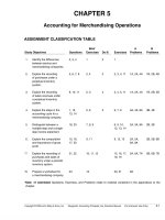
ASSIGNMENT CLASSIFICATION TABLE
Brief
Exercises

Exercises

A
Problems

B
Problems

1, 2, 3,
4, 5

1

1, 2

1A

1B

Explain the accounting
for inventories and apply
the inventory cost flow
methods.

5, 7, 8,

9, 10,

2, 3, 4

3, 4, 5,
6, 7, 8

2A, 3A, 4A,
5A, 6A, 7A

2B, 3B, 4B,
5B, 6B, 7B

3.

Explain the financial
effects of the inventory
cost flow assumptions.

6, 11, 12

5, 6

3, 6, 7, 8

2A, 3A, 4A,
5A, 6A, 7A

2B, 3B, 4B,
5B, 6B, 7B

4.

Explain the lower-ofcost-or-market basis of
accounting for inventories.

13, 14, 15

7

9, 10

5.

Indicate the effects of
inventory errors on the
financial statements.

16

8

11, 12

6.

Compute and interpret
the inventory turnover
ratio.

17, 18

9

13, 14

*7. Apply the inventory cost
flow methods to perpetual
inventory records.

19, 20

10

15, 16, 17

8A, 9A

8B, 9B

*8. Describe the two methods
of estimating inventories.

21, 22,
23, 24

11, 12

18, 19, 20

10A, 11A

10B, 11B

Study Objectives

Questions

1.

Describe the steps in
determining inventory
quantities.

2.

*Note: All asterisked Questions, Exercises, and Problems relate to material contained in the appendices
to the chapter.

6-1


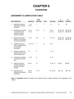
ASSIGNMENT CHARACTERISTICS TABLE
Problem
Number

Description

Difficulty
Level

Time Allotted
(min.)

1A

Determine items and amounts to be recorded in inventory.

Moderate

15–20

2A

Determine cost of goods sold and ending inventory using
FIFO, LIFO, and average-cost with analysis.

Simple

30–40

3A

Determine cost of goods sold and ending inventory using
FIFO, LIFO, and average-cost with analysis.

Simple

30–40

4A

Compute ending inventory, prepare income statements,
and answer questions using FIFO and LIFO.

Moderate

30–40

5A

Calculate ending inventory, cost of goods sold, gross profit,
and gross profit rate under periodic method; compare
results.

Moderate

30–40

6A

Compare specific identification, FIFO, and LIFO under
periodic method; use cost flow assumption to influence
earnings.

Moderate

20–30

7A

Compute ending inventory, prepare income statements,
and answer questions using FIFO and LIFO.

Moderate

30–40

*8A

Calculate cost of goods sold and ending inventory for
FIFO, average-cost, and LIFO, under the perpetual
system; compare gross profit under each assumption.

Moderate

30–40

*9A

Determine ending inventory under a perpetual inventory
system.

Moderate

40–50

*10A

Estimate inventory loss using gross profit method.

Moderate

30–40

*11A

Compute ending inventory using retail method.

Moderate

20–30

1B

Determine items and amounts to be recorded in inventory.

Moderate

15–20

2B

Determine cost of goods sold and ending inventory using
FIFO, LIFO, and average-cost with analysis.

Simple

30–40

3B

Determine cost of goods sold and ending inventory using
FIFO, LIFO, and average-cost with analysis.

Simple

30–40

4B

Compute ending inventory, prepare income statements,
and answer questions using FIFO and LIFO.

Moderate

30–40

5B

Calculate ending inventory, cost of goods sold, gross profit,
and gross profit rate under periodic method; compare
results.

Moderate

30–40

6B

Compare specific identification, FIFO, and LIFO under
periodic method; use cost flow assumption to justify
price increase.

Moderate

20–30

6-2


ASSIGNMENT CHARACTERISTICS TABLE (Continued)
Problem
Number

Difficulty
Level

Time Allotted
(min.)

Compute ending inventory, prepare income statements,
and answer questions using FIFO and LIFO.

Moderate

30–40

*8B

Calculate cost of goods sold and ending inventory under
LIFO, FIFO, and average-cost, under the perpetual system;
compare gross profit under each assumption.

Moderate

30–40

*9B

Determine ending inventory under a perpetual inventory
system.

Moderate

40–50

*10B

Compute gross profit rate and inventory loss using gross
profit method.

Moderate

30–40

*11B

Compute ending inventory using retail method.

Moderate

20–30

7B

Description

6-3


6-4

Explain the accounting for
inventories and apply the
inventory cost flow methods.

Explain the financial effects of the
inventory cost flow assumptions.

Explain the lower-of-cost-or-market
basis of accounting for inventories.

Indicate the effects of inventory
errors on the financial statements.

Compute and interpret the inventory
turnover ratio.

Apply the inventory cost flow

methods to perpetual inventory
records.

Describe the two methods of
estimating inventories.

2.

3.

4.

5.

6.

*7.

*8.

Broadening Your Perspective

Describe the steps in determining
inventory quantities.

1.

Study Objective

E6-18 P6-11A

E6-19 P6-10B
E6-20 P6-11B
P6-10A

P6-8A
P6-9A
P6-8B
P6-9B

Communication
Exploring the
Web

E6-14 Q6-18
BE6-9

Financial Reporting
Decision Making
Across the
Organization

Q6-23
Q6-24
BE6-11
BE6-12

BE6-10
E6-15
E6-16
E6-17

Q6-19
Q6-20

Q6-21
Q6-22

BE6-9
E6-13

Q6-17

E6-11
E6-12

All About You
Ethics Case
Comp. Analysis

E6-16
E6-17
P6-8A
P6-8B

BE6-7
E6-9
E6-10

Q6-13

Q6-16
BE6-8

E6-3
P6-5A
P6-5B
P6-6A
P6-6B

P6-5B E6-3
P6-6A P6-4A
P6-6B P6-4B
P6-7A
P6-7B

P6-2A
P6-2B
P6-3A
P6-3B
P6-5A

BE6-5
BE6-6
E6-6
E6-7
E6-8

Q6-6
Q6-11
Q6-12

Q6-14
Q6-15

E6-3
E6-4
P6-5A
P6-5B

Evaluation

E6-3
E6-4
P6-4A
P6-4B
P6-7A
P6-7B

P6-1A
P6-1B

Synthesis

P6-5A
P6-5B
P6-6A
P6-6B

E6-1
E6-2

Analysis

E6-7
E6-8
P6-2A
P6-3A
P6-2B
P6-3B

Q6-7
Q6-9

Q6-8
Q6-10
BE6-5

Q6-4 Q6-5
BE6-1 E6-1

Application

Q6-5
BE6-2
BE6-3
BE6-4
E6-5
E6-6

Q6-1

Q6-3

Q6-2

Knowledge Comprehension

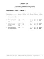
Correlation Chart between Bloom’s Taxonomy, Study Objectives and End-of-Chapter Exercises and Problems

BLOOM’S TAXONOMY TABLE


ANSWERS TO QUESTIONS
1.

Agree. Effective inventory management is frequently the key to successful business operations.
Management attempts to maintain sufficient quantities and types of goods to meet expected
customer demand. It also seeks to avoid the cost of carrying inventories that are clearly in excess
of anticipated sales.

2.

Inventory items have two common characteristics: (1) they are owned by the company and (2) they
are in a form ready for sale in the ordinary course of business.

3.

Taking a physical inventory involves actually counting, weighing or measuring each kind of
inventory on hand. Retailers, such as a hardware store, generally have thousands of different
items to count. This is normally done when the store is closed.

4.

(a) (1)

5.

Inventoriable costs are $3,020 (invoice cost $3,000 + freight charges $50 – purchase discounts
$30). The amount paid to negotiate the purchase is a buying cost that normally is not included in
the cost of inventory because of the difficulty of allocating these costs. Buying costs are
expensed in the year incurred.

6.

There are three distinguishing features in the income statement of a merchandising company:
(1) a sales revenues section, (2) a cost of goods sold section, and (3) gross profit.

7.

Actual physical flow may be impractical because many items are indistinguishable from one
another. Actual physical flow may be inappropriate because management may be able to
manipulate net income through specific identification of items sold.

8.

The major advantage of the specific identification method is that it tracks the actual physical flow
of the goods available for sale. The major disadvantage is that management could manipulate
net income.

9.

No. Selection of an inventory costing method is a management decision. However, once a method
has been chosen, it should be consistently applied.

The goods will be included in Reeves Company’s inventory if the terms of sale are
FOB destination.
(2) They will be included in Cox Company’s inventory if the terms of sale are FOB shipping
point.
(b) Reeves Company should include goods shipped to a consignee in its inventory. Goods held
by Reeves Company on consignment should not be included in inventory.

10.

(a) FIFO.
(b) Average-cost.
(c) LIFO.

11.

Plato Company is using the FIFO method of inventory costing, and Cecil Company is using the
LIFO method. Under FIFO, the latest goods purchased remain in inventory. Thus, the inventory
on the balance sheet should be close to current costs. The reverse is true of the LIFO method.
Plato Company will have the higher gross profit because cost of goods sold will include a higher
proportion of goods purchased at earlier (lower) costs.

6-5


Questions Chapter 6 (Continued)
12. Casey Company may experience severe cash shortages if this policy continues. All of its net
income is being paid out as dividends, yet some of the earnings must be reinvested in inventory

to maintain inventory levels. Some earnings must be reinvested because net income is
computed with cost of goods sold based on older, lower costs while the inventory must be
replaced at current, higher costs. Because of this factor, net income under FIFO is sometimes
referred to as “phantom profits.”
13. Peter should know the following:
(a) A departure from the cost basis of accounting for inventories is justified when the value of
the goods is lower than its cost. The writedown to market should be recognized in the period
in which the price decline occurs.
(b) Market means current replacement cost, not selling price. For a merchandising company,
market is the cost at the present time from the usual suppliers in the usual quantities.
14. Garitson Music Center should report the CD players at $380 each for a total of $1,900. $380
is the current replacement cost under the lower-of-cost-or-market basis of accounting for inventories.
A decline in replacement cost usually leads to a decline in the selling price of the item. Valuation
at LCM is conservative.
15. Ruthie Stores should report the toasters at $27 each for a total of $540. The $27 is the lower of cost
or market. It is used because it is the lower of the inventory’s cost and current replacement cost.
16. (a) Mintz Company’s 2007 net income will be understated $7,000; (b) 2008 net income will be
overstated $7,000; and (c) the combined net income for the two years will be correct.
17. Willingham Company should disclose: (1) the major inventory classifications, (2) the basis of
accounting (cost or lower of cost or market), and (3) the costing method (FIFO, LIFO, or average).
18. An inventory turnover that is too high may indicate that the company is losing sales opportunities
because of inventory shortages. Inventory outages may also cause customer ill will and result in
lost future sales.
*19. Disagree. The results under the FIFO method are the same but the results under the LIFO
method are different. The reason is that the pool of inventoriable costs (cost of goods available
for sale) is not the same. Under a periodic system, the pool of costs is the goods available for
sale for the entire period, whereas under a perpetual system, the pool is the goods available for
sale up to the date of sale.
*20. In a periodic system, the average is a weighted average based on total goods available for sale for the
period. In a perpetual system, the average is a moving average of goods available for sale after

each purchase.
*21. Inventories must be estimated when: (1) management wants monthly or quarterly financial
statements but a physical inventory is only taken annually and (2) a fire or other type of casualty
makes it impossible to take a physical inventory.

6-6


Questions Chapter 6 (Continued)
*22. In the gross profit method, the average is the gross profit rate, which is gross profit divided by net
sales. The rate is often based on last year’s actual rate. The gross profit rate is applied to net sales
in using the gross profit method.
In the retail inventory method, the average is the cost-to-retail ratio, which is the goods available
for sale at cost divided by the goods available for sale at retail. The ratio is based on current year
data and is applied to the ending inventory at retail.
*23. The estimated cost of the ending inventory is $40,000:
Net sales ......................................................................................................................................
Less: Gross profit ($400,000 X 35%) ....................................................................................
Estimated cost of goods sold ...................................................................................................

$400,000
140,000
$260,000

Cost of goods available for sale ..............................................................................................
Less: Cost of goods sold..........................................................................................................
Estimated cost of ending inventory.........................................................................................

$300,000
260,000

$ 40,000

*24. The estimated cost of the ending inventory is $28,000:

 $84,000 
 $120,000 

Cost-to-retail ratio:

70% =

Ending inventory at retail:

$40,000 = ($120,000 – $80,000)

Ending inventory at cost:

$28,000 = ($40,000 X 70%)

6-7


SOLUTIONS TO BRIEF EXERCISES
BRIEF EXERCISE 6-1
(a) Ownership of the goods belongs to the consignor (Smart). Thus, these
goods should be included in Smart’s inventory.
(b) The goods in transit should not be included in the inventory count
because ownership by Smart does not occur until the goods reach
the buyer.
(c) The goods being held belong to the customer. They should not be

included in Smart’s inventory.
(d) Ownership of these goods rests with the other company (the consignor).
Thus, these goods should not be included in the physical inventory.

BRIEF EXERCISE 6-2
The items that should be included in inventoriable costs are:
(a)
(b)
(c)
(e)

Freight-in
Purchase Returns and Allowances
Purchases
Purchase Discounts

BRIEF EXERCISE 6-3
(a) The ending inventory under FIFO consists of 200 units at $8 + 160 units
at $7 for a total allocation of $2,720 or ($1,600 + $1,120).
(b) The ending inventory under LIFO consists of 300 units at $6 + 60 units
at $7 for a total allocation of $2,220 or ($1,800 + $420).

6-8


BRIEF EXERCISE 6-4
Average unit cost is $6.89 computed as follows:
300 X $6 = $1,800
400 X $7 = 2,800
200 X $8 = 1,600

900
$6,200
$6,200 ÷ 900 = $6.89 (rounded).
The cost of the ending inventory is $2,480 or (360 X $6.89).
BRIEF EXERCISE 6-5
(a)
(b)
(c)
(d)

FIFO would result in the highest net income.
FIFO would result in the highest ending inventory.
LIFO would result in the lowest income tax expense (because it would
result in the lowest net income).
Average-cost would result in the most stable income over a number
of years because it averages out any big changes in the cost of inventory.

BRIEF EXERCISE 6-6
Cost of good sold under:
Purchases

Cost of goods available for sale
Less: Ending inventory
Cost of goods sold

LIFO
$6 X 100
$7 X 200
$8 X 150
$ 3,200

$ 1,160
$ 2,040

FIFO
$6 X 100
$7 X 200
$8 X 150
$ 3,200
$ 1,410
$ 1,790

Since the cost of goods sold is $250 less under FIFO ($2,040 – $1,790) that
is the amount of the phantom profit. It is referred to as “phantom profit”
because FIFO matches current selling prices with old inventory costs. To
replace the units sold, the company will have to pay the current price of $8
per unit, rather than the $6 per unit which some of the units were priced at
under FIFO. Therefore, profit under LIFO is more representative of what the
company can expect to earn in future periods.

6-9


BRIEF EXERCISE 6-7
Inventory Categories
Cameras
Camcorders
VCRs
Total valuation

Cost

$12,000
9,500
14,000

Market
$12,100
9,700
12,800

LCM
$12,000
9,500
12,800
$34,300

BRIEF EXERCISE 6-8
The understatement of ending inventory caused cost of goods sold to be
overstated $10,000 and net income to be understated $10,000. The correct
net income for 2008 is $100,000 or ($90,000 + $10,000).
Total assets in the balance sheet will be understated by the amount that
ending inventory is understated, $10,000.

BRIEF EXERCISE 6-9

Inventory turnover:

Days in inventory:

$270,000
$270,000

=
= 5.4
( $60,000 + $40,000 ) ÷ 2 $50,000

365
= 67.6 days
5.4

*BRIEF EXERCISE 6-10
(1) FIFO Method

Date
May 7
June 1
July 28
Aug. 27

Purchases
(50 @ $10) $500
(30 @ $13)

Product E2-D2
Cost of
Goods Sold
(30 @ $10)

$300

(20 @ $10)
(20 @ $13)

} $460

$390

6-10

Balance
(50 @ $10)
$500
(20 @ $10)
$200
(20 @ $10)
} $590
(30 @ $13)
(10 @ $13)

$130


*BRIEF EXERCISE 6-10 (Continued)
(2) LIFO Method

Date
May 7
June 1
July 28

Purchases
(50 @ $10) $500

(30 @ $13)

Product E2-D2
Cost of
Goods Sold
(30 @ $10)

$300

(30 @ $13)
(10 @ $10)

} $490

$390

Aug. 27

Balance
(50 @ $10)
$500
(20 @ $10)
$200
(20 @ $10)
} $590
(30 @ $13)
(10 @ $10)

$100

(3) Average-Cost

Date
May 7
June 1
July 28
Aug. 27

Purchases
(50 @ $10) $500

Product E2-D2
Cost of
Goods Sold
(30 @ $10)

(30 @ $13)

$300

$390
(40 @ $11.80) $472

Balance
(50 @ $10)
$500
(20 @ $10)
$200
(50 @ $11.80)* $590
(10 @ $11.80) $118

*($200 + $390) ÷ 50
*BRIEF EXERCISE 6-11
(1) Net sales
Less: Estimated gross profit (35% X $330,000)
Estimated cost of goods sold

$330,000
115,500
$214,500

(2) Cost of goods available for sale
Less: Estimated cost of goods sold
Estimated cost of ending inventory

$230,000
214,500
$ 15,500

*BRIEF EXERCISE 6-12
At Cost
$35,000

Goods available for sale
Net sales
Ending inventory at retail

Cost-to-retail ratio = ($35,000 ÷ $50,000) = 70%
Estimated cost of ending inventory = ($10,000 X 70%) = $7,000
6-11

At Retail
$50,000
40,000
$10,000


SOLUTIONS TO EXERCISES
EXERCISE 6-1
Ending inventory—physical count....................................................
1. No effect—title passes to purchaser upon shipment
when terms are FOB shipping point....................................
2. No effect—title does not transfer to Lima until
goods are received ....................................................................
3. Add to inventory: Title passed to Lima when goods
were shipped ...............................................................................
4. Add to inventory: Title remains with Lima until
purchaser receives goods ......................................................
5. The goods did not arrive prior to year-end. The goods,
therefore, cannot be included in the inventory................
Correct inventory ....................................................................................

$297,000
0
0
22,000
35,000
(44,000)
$310,000

EXERCISE 6-2
Ending inventory—as reported ..........................................................
1. Subtract from inventory: The goods belong to
Superior Corporation. Strawser is merely holding
them as a consignee ................................................................
2. No effect—title does not pass to Strawser until
goods are received (Jan. 3)....................................................
3. Subtract from inventory: Office supplies should
be carried in a separate account. They are not
considered inventory held for resale..................................
4. Add to inventory: The goods belong to Strawser
until they are shipped (Jan. 1)...............................................
5. Add to inventory: District Sales ordered goods
with a cost of $8,000. Strawser should record the
corresponding sales revenue of $10,000. Strawser’s
decision to ship extra “unordered” goods does not
constitute a sale. The manager’s statement that District
could ship the goods back indicates that Strawser knows
this over-shipment is not a legitimate sale. The manager
acted unethically in an attempt to improve Strawser’s
reported income by over-shipping ......................................

6-12

$740,000

(250,000)
0

(17,000)

30,000

52,000


EXERCISE 6-2 (Continued)
6.

Subtract from inventory: GAAP require that inventory
be valued at the lower of cost or market. Obsolete parts
should be adjusted from cost to zero if they have no
other use..........................................................................................
Correct inventory........................................................................................

(40,000)
$515,000

EXERCISE 6-3
(a)

FIFO Cost of Goods Sold
(#1012) $100 + (#1045) $90 = $190

(b)

It could choose to sell specific units purchased at specific costs if it
wished to impact earnings selectively. If it wished to minimize earnings
it would choose to sell the units purchased at higher costs—in which
case the Cost of Goods Sold would be $190. If it wished to maximize
earnings it would choose to sell the units purchased at lower costs—in

which case the cost of goods sold would be $170.

(c)

I recommend they use the FIFO method because it produces a more
appropriate balance sheet valuation and reduces the opportunity to
manipulate earnings.
(The answer may vary depending on the method the student chooses.)

EXERCISE 6-4
FIFO
Beginning inventory (26 X $97).....................................................
$ 2,522
Purchases
Sept. 12 (45 X $102).................................................................. $4,590
Sept. 19 (20 X $104).................................................................. 2,080
Sept. 26 (50 X $105).................................................................. 5,250 11,920
Cost of goods available for sale...................................................
14,442
Less: Ending inventory (20 X $105) ...........................................
2,100
Cost of goods sold............................................................................
$12,342

6-13


EXERCISE 6-4 (Continued)

Date

9/1
9/12
9/19
9/26

Units
26
45
20
30
121

Proof
Unit Cost
$ 97
102
104
105

Total Cost
$ 2,522
4,590
2,080
3,150
$12,342

LIFO
Cost of goods available for sale.................................................................... $14,442
Less: Ending inventory (20 X $97)...............................................................
1,940

Cost of goods sold............................................................................................. $12,502

Date
9/26
9/19
9/12
9/1

Units
50
20
45
6
121

Proof
Unit Cost
$105
104
102
97

Total Cost
$ 5,250
2,080
4,590
582
$12,502

(b)

FIFO $2,100 (ending inventory) + $12,342 (COGS) = $14,442
LIFO $1,940 (ending inventory) + $12,502 (COGS) = $14,442

}

Cost of
goods
available
for sale

Under both methods, the sum of the ending inventory and cost of goods sold
equals the same amount, $14,442, which is the cost of goods available for sale.
EXERCISE 6-5
FIFO
Beginning inventory (30 X $8) .......................................................
Purchases
May 15 (25 X $11) ......................................................................
May 24 (35 X $12) ......................................................................
Cost of goods available for sale...................................................
Less: Ending inventory (25 X $12)..............................................
Cost of goods sold............................................................................
6-14

$240
$275
420

695
935
300

$635


EXERCISE 6-5 (Continued)

Date
5/1
5/15
5/24

Units
30
25
10

Proof
Unit Cost
$ 8
11
12

Total Cost
$240
275
120
$635

LIFO
Cost of goods available for sale....................................................................
Less: Ending inventory (25 X $8) .................................................................

Cost of goods sold.............................................................................................

Date
5/24
5/15
5/1

Units
35
25
5

Proof
Unit Cost
$12
11
8

$935
200
$735

Total Cost
$420
275
40
$735

EXERCISE 6-6
(a)

FIFO
Beginning inventory (200 X $5).....................................
Purchases
June 12 (300 X $6) ....................................................
June 23 (500 X $7) ....................................................
Cost of goods available for sale...................................
Less: Ending inventory (120 X $7)..............................
Cost of goods sold............................................................
LIFO
Cost of goods available for sale...................................
Less: Ending inventory (120 X $5)..............................
Cost of goods sold............................................................

6-15

$1,000
$1,800
3,500

5,300
6,300
840
$5,460
$6,300
600
$5,700


EXERCISE 6-6 (Continued)

(b) The FIFO method will produce the higher ending inventory because
costs have been rising. Under this method, the earliest costs are
assigned to cost of goods sold and the latest costs remain in ending
inventory. For Yount Company, the ending inventory under FIFO is
$840 or (120 X $7) compared to $600 or (120 X $5) under LIFO.
(c) The LIFO method will produce the higher cost of goods sold for Yount
Company. Under LIFO the most recent costs are charged to cost of
goods sold and the earliest costs are included in the ending inventory.
The cost of goods sold is $5,700 or [$6,300 – (120 X $5)] compared to
$5,460 or ($6,300 – $840) under FIFO.
EXERCISE 6-7
(a)

1.

2.

3.

FIFO
Beginning inventory ..................................................
Purchases......................................................................
Cost of goods available for sale ............................
Less: ending inventory (80 X $130) .....................
Cost of goods sold .....................................................

$10,000
26,000
36,000
(10,400)

$25,600

LIFO
Beginning inventory ..................................................
Purchases......................................................................
Cost of goods available for sale ............................
Less: ending inventory (80 X $100) .....................
Cost of goods sold .....................................................

$10,000
26,000
36,000
(8,000)
$28,000

AVERAGE
Beginning inventory ..................................................
Purchases......................................................................
Cost of goods available for sale ............................
Less: ending inventory (80 X $120) .....................
Cost of goods sold .....................................................

$10,000
26,000
36,000
(9,600)
$26,400

(b) The use of FIFO would result in the highest net income since the earlier
lower costs are matched with revenues.

(c) The use of FIFO would result in inventories approximating current cost in
the balance sheet, since the more recent units are assumed to be on hand.
(d) The use of LIFO would result in Jones paying the least taxes in the
first year since income will be lower.

6-16


EXERCISE 6-8
(a)

Total Units
Cost of Goods
Available for Sale ÷ Available for Sale
1,000
$6,300
Ending inventory (120 X $6.30)
Cost of goods sold (880 X $6.30)

=

Weighted Average
Unit Cost
$6.30

$ 756
5,544

(b) Ending inventory is lower than FIFO ($840) and higher than LIFO
($600). In contrast, cost of goods sold is higher than FIFO ($5,460)

and lower than LIFO ($5,700).
(c) The average-cost method uses a weighted-average unit cost, not a simple
average of unit costs.
EXERCISE 6-9
Lower
of Cost
or Market:

Cost

Market

Cameras
Minolta
Canon
Total

$ 850
900
1,750

$ 780
912
1,692

$ 780
900

Light meters
Vivitar

Kodak
Total
Total inventory

1,500
1,680
3,180
$4,930

1,380
1,890
3,270
$4,962

1,380
1,680
$4,740

Market
$ 7,100
10,350
9,750
$27,200

Lower
of Cost
or Market:
$ 6,500
10,350
9,750

$26,600

EXERCISE 6-10

VCRs
DVD players
Ipods
Total inventory

Cost
$ 6,500
11,250
10,000
$27,750

6-17


EXERCISE 6-11

Beginning inventory ...................................................
Cost of goods purchased .........................................
Cost of goods available for sale.............................
Corrected ending inventory .....................................
Cost of goods sold......................................................
a

$30,000 – $3,000 = $27,000.

b

2008

2009

$ 20,000
150,000
170,000
a
27,000
$143,000

$ 27,000
175,000
202,000
41,000b
$161,000

$35,000 + $6,000 = $41,000.

EXERCISE 6-12
(a)
Sales ............................................................................
Cost of goods sold
Beginning inventory.......................................
Cost of goods purchased.............................
Cost of goods available for sale ................
Ending inventory ($44,000 – $5,000).........
Cost of goods sold .........................................
Gross profit ...............................................................

2008
$210,000

2009
$250,000

32,000
173,000
205,000
39,000
166,000
$ 44,000

39,000
202,000
241,000
52,000
189,000
$ 61,000

(b) The cumulative effect on total gross profit for the two years is zero as
shown below:
Incorrect gross profits:
Correct gross profits:
Difference

$49,000 + $56,000 = $105,000
$44,000 + $61,000 = 105,000
$

0

(c) Dear Mr./Ms. President:
Because your ending inventory of December 31, 2008 was overstated
by $5,000, your net income for 2008 was overstated by $5,000. For 2009
net income was understated by $5,000.
In a periodic system, the cost of goods sold is calculated by deducting
the cost of ending inventory from the total cost of goods you have
available for sale in the period. Therefore, if this ending inventory figure
is overstated, as it was in December 2008, then the cost of goods sold
is understated and therefore net income will be overstated by that
amount. Consequently, this overstated ending inventory figure goes on
to become the next period’s beginning inventory amount and is a part
of the total cost of goods available for sale. Therefore, the mistake
repeats itself in the reverse.
6-18


EXERCISE 6-12 (Continued)
The error also affects the balance sheet at the end of 2008. The inventory reported in the balance sheet is overstated; therefore, total assets
are overstated. The overstatement of the 2008 net income results in the
capital account balance being overstated. The balance sheet at the end
of 2009 is correct because the overstatement of the capital account at
the end of 2008 is offset by the understatement of the 2009 net income
and the inventory at the end of 2009 is correct.
Thank you for allowing me to bring this to your attention. If you have
any questions, please contact me at your convenience.
Sincerely,
EXERCISE 6-13

Inventory
turnover

2007

2008

$900,000
($100,000 + $300,000) ÷ 2

$1,120,000
($300,000 + $400,000) ÷ 2

$900,000
$200,000
Days in
inventory
Gross
profit rate

365
4.5

= 4.5

= 81.1 days

$1,200,000 – $900,000
= .25
$1,200,000

$1,120,000
$350,000
365
3.2

= 3.2

= 114.1 days

$1,600,000 – $1,120,000
= .30
$1,600,000

2009
$1,300,000
($400,000 + $480,000) ÷ 2
$1,300,000
$440,000
365
2.95

= 2.95

= 123.7 days

$1,900,000 – $1,300,000
= .32
$1,900,000

The inventory turnover ratio decreased by approximately 34% from 2007 to
2009 while the days in inventory increased by almost 53% over the same
time period. Both of these changes would be considered negative since it’s
better to have a higher inventory turnover with a correspondingly lower days
in inventory. However, Santo’s Photo gross profit rate increased by 28%
from 2007 to 2009, which is a positive sign.

6-19


EXERCISE 6-14
(a)
Inventory Turnover

O’Brien Company

Weinberg Company

$190,000
($45,000 + $55,000)/2
= 3.80

$292,000
($71,000 + $69,000)/2
= 4.17

365/3.80 = 96 days

365/4.17 = 88 days

Days in Inventory
(b)

Weinberg Company is moving its inventory more quickly, since its inventory turnover is higher, and its days in inventory is lower.

*EXERCISE 6-15
(1)
Date
Purchases
Jan. 1
8
10 (6 @ $660) $3,960
15

Purchases

Jan. 1
8
10 (6 @ $660) $3,960
15

(2 @ $600) $1,200

(1 @ $600)
(3 @ $660) $2,580

(2)
Date

FIFO

Cost of Goods Sold

LIFO
Cost of Goods Sold
(2 @ $600) $1,200

(4 @ $660) $2,640

6-20

Balance
(3 @ $600) $1,800
(1 @ $600)
600
(1 @ $600)
(6 @ $660)
4,560
(3 @ $660)

1,980

Balance
(3 @ $600) $1,800
(1 @ $600)
600
(1 @ $600)
(6 @ $660)
4,560
(1 @ $600)
(2 @ $660)

1,920


*EXERCISE 6-15 (Continued)
(3)

AVERAGE-COST
Date
Purchases
Cost of Goods Sold
Jan. 1
8
(2 @ $600)
$1,200
10 (6 @ $660) $3,960
15
(4 @ $651.43) $2,606

Balance
(3 @ $600)
$1,800
(1 @ $600)
600
(7 @ $651.43)* 4,560
(3 @ $651.43) 1,954

*Average-cost = ($600 + $3,960) ÷ 7 = $651.43 (rounded)
*EXERCISE 6-16
(a)

The cost of goods available for sale is:
June 1 Inventory
200 @ $5
June 12 Purchase
300 @ $6
June 23 Purchase
500 @ $7
Total cost of goods available for sale

Date
June 1
June 12

Purchases
(300 @ $6) $1,800

June 15
June 23
June 27

FIFO
Cost of Goods Sold

$1,000
1,800
3,500
$6,300
Balance
(200 @ $5)
$1,000

(200 @ $5)
$2,800
(300 @ $6)

}

(200 @ $5)
(200 @ $6)

$1,000
1,200

(500 @ $7) $3,500
(100 @ $6)
(380 @ $7)

600
2,660
$5,460

(100 @ $6)
(100 @ $6)
(500 @ $7)
(120 @ $7)

$ 600

}

$4,100

$ 840

Ending inventory: $840. Cost of goods sold: $6,300 – $840 = $5,460.

6-21


*EXERCISE 6-16 (Continued)

Date
Purchases
June 1
June 12 (300 @ $6) $1,800
June 15

LIFO
Cost of Goods Sold

}

(300 @ $6)
(100 @ $5)

$1,800
$ 500

June 23 (500 @ $7) $3,500
June 27

Balance

(200 @ $5)
$1,000
(200 @ $5)
$2,800
(300 @ $6)

(480 @ $7)

$3,360
$5,660

(100 @ $5)
(100 @ $5)
(500 @ $7)
(100 @ $5)
( 20 @ $7)

$ 500

}
}

$4,000
$ 640

Ending inventory: $640. Cost of goods sold: $6,300 – $640 = $5,660.

Date
June 1
June 12

June 15
June 23
June 27

Purchases

Moving-Average
Cost of Goods Sold

(300 @ $6) $1,800
(400 @ $5.60)

$2,240

(500 @ $7) $3,500
(480 @ $6.767) $3,248
$5,488

Balance
(200 @ $5)
$1,000
(500 @ $5.60) $2,800
(100 @ $5.60) $ 560
(600 @ $6.767) $4,060
(120 @ $6.767) $ 812

Ending inventory: $812. Cost of goods sold: $6,300 – $812 = $5,488.
(b)

FIFO gives the same ending inventory and cost of goods sold values

under both the periodic and perpetual inventory system. LIFO and
average give different ending inventory and cost of goods sold values
under the periodic and perpetual inventory systems, due to the Last-in,
First-out assumption being applied to a different pool of costs.

(c)

The simple average would be [($5 + $6 + $7) ÷ 3)] or $6. However, the
average-cost method uses a weighted-average unit cost that changes
each time a purchase is made rather than a simple average.

6-22


*EXERCISE 6-17
(a)

Date
9/1
9/5
9/12

FIFO
Cost of
Goods Sold

Purchases

(12 @ $ 97) $1,164
(45 @ $102)

$4,590

9/16

(14 @ $ 97)
(36 @ $102) $5,030

9/19

(20 @ $104)

$2,080

9/26

(50 @ $105)

$5,250

9/29

Date
9/1
9/5
9/12

( 9 @ $102)
(20 @ $104)
(30 @ $105) $6,148

LIFO
Cost of
Goods Sold

Purchases

(12 @ $ 97) $1,164
(45 @ $102)

$4,590

9/16
9/19
9/26
9/29

(45 @ $102)
( 5 @ $ 97) $5,075
(20 @ $104)
(50 @ $105)

$2,080
$5,250
(50 @ $105)
( 9 @ $104) $6,186

6-23

Balance
(26 @ $ 97) $2,522

(14 @ $ 97) $1,358
(14 @ $ 97)
(45 @ $102) $5,948
( 9 @ $102) $ 918
( 9 @ $102)
(20 @ $104) $2,998
( 9 @ $102)
(20 @ $104)
(50 @ $105) $8,248
(20 @ $105) $2,100

Balance
(26 @ $ 97) $2,522
(14 @ $ 97) $1,358
(14 @ $ 97)
(45 @ $102) $5,948
( 9 @ $ 97)
( 9 @ $ 97)
(20 @ $104)
( 9 @ $ 97)
(20 @ $104)
(50 @ $105)
( 9 @ $ 97)
(11 @ $104)

$ 873
$2,953
$8,203
$2,017

*EXERCISE 6-17 (Continued)

Date
9/1
9/5
9/12
9/16
9/19
9/26
9/29

Purchases

Average-Cost
Cost of
Goods Sold
(12 @ $97)

$1,164

(50 @ $100.81)

$5,041*

(59 @ $104.27)

$6,152*

(45 @ $102) $4,590

(20 @ $104) $2,080
(50 @ $105) $5,250

Balance
(26 @ $97)
(14 @ $97)
(59 @ $100.81)a
( 9 @ $100.81)
(29 @ $103.00)b
(79 @ $104.27)c
(20 @ $104.27)

$2,522
$1,358
$5,948
$ 907
$2,987
$8,237
$2,085

*Rounded
a
$5,948 ÷ 59 = $100.81
b
$2,987 ÷ 29 = $103.00
c
$8,237 ÷ 79 = $104.27
(b)
Periodic
$2,100

$1,940

Ending Inventory FIFO
Ending Inventory LIFO

(c)

Perpetual
$2,100
$2,017

FIFO yields the same ending inventory value under both the periodic
and perpetual inventory system.
LIFO yields different ending inventory values when using the periodic
versus perpetual inventory system.

*EXERCISE 6-18
(a)

Sales ..................................................................................
Cost of goods sold
Inventory, November 1 .....................................
Cost of goods purchased ................................
Cost of goods available for sale....................
Inventory, December 31 ...................................
Cost of goods sold..................................
Gross profit .....................................................................
Gross profit rate $320,000/$800,000 = 40%

6-24

$800,000
$100,000
500,000
600,000
(120,000)
480,000
$320,000


*EXERCISE 6-18 (Continued)
(b) Sales ......................................................................................................
Less: Estimated gross profit (40% X $1,000,000) ..................
Estimated cost of goods sold .......................................................

$1,000,000
400,000
$ 600,000

Beginning inventory .........................................................................
Cost of goods purchased ...............................................................
Cost of goods available for sale...................................................
Less: Estimated cost of goods sold ..........................................
Estimated cost of ending inventory ............................................

$120,000
610,000
730,000
600,000
$130,000

*EXERCISE 6-19
(a) Net sales ($51,000 – $1,000)...........................................................
Less: Estimated gross profit (40% X $50,000)........................
Estimated cost of goods sold .......................................................

$50,000
20,000
$30,000

Beginning inventory .........................................................................
Cost of goods purchased ($31,200 – $1,400 + $1,200)..........
Cost of goods available for sale...................................................
Less: Estimated cost of goods sold ..........................................
Estimated cost of merchandise lost ...........................................

$20,000
31,000
51,000
30,000
$21,000

(b) Net sales ...............................................................................................
Less: Estimated gross profit (30% X $50,000)........................
Estimated cost of goods sold .......................................................

$50,000
15,000
$35,000

Beginning inventory .........................................................................
Cost of goods purchased ...............................................................
Cost of goods available for sale...................................................
Less: Estimated cost of goods sold ..........................................
Estimated cost of merchandise lost ...........................................

$30,000
31,000
61,000
35,000
$26,000

6-25