Solution manual cost accounting 14e by horngren chapter 19

To download more slides, ebook, solutions and test bank, visit

CHAPTER 19
BALANCED SCORECARD:
QUALITY, TIME, AND THE THEORY OF CONSTRAINTS
19-1 Quality costs (including the opportunity cost of lost sales because of poor quality) can be
as much as 10% to 20% of sales revenues of many organizations. Quality-improvement
programs can result in substantial cost savings and higher revenues and market share from
increased customer satisfaction.
19-2 Design quality refers to how closely the characteristics of a product or service meet the
needs and wants of customers. Conformance quality refers to the performance of a product or
service relative to its design and product specifications.
19-3 Exhibit 19-1 of the text lists the following six line items in the prevention costs category:
design engineering; process engineering; supplier evaluations; preventive equipment
maintenance; quality training; and testing of new materials.
19-4 An internal failure cost differs from an external failure cost on the basis of when the
nonconforming product is detected. Internal failure costs are costs incurred on a defective
product before a product is shipped to a customer, whereas external failure costs are costs
incurred on a defective product after a product is shipped to a customer.
19-5 Three methods that companies use to identify quality problems are: (a) a control chart
which is a graph of a series of successive observations of a particular step, procedure, or
operation taken at regular intervals of time; (b) a Pareto diagram, which is a chart that indicates
how frequently each type of failure (defect) occurs, ordered from the most frequent to the least
frequent; and (c) a cause-and-effect diagram, which helps identify potential causes of defects
using a diagram that resembles the bone structure of a fish.
19-6 No, companies should emphasize financial as well as nonfinancial measures of quality,
such as yield and defect rates. Nonfinancial measures are not directly linked to bottom-line
performance but they indicate and direct attention to the specific areas that need improvement to
improve the bottom line. Tracking nonfinancial measures over time directly reveals whether
these areas have, in fact, improved over time. Nonfinancial measures are easy to quantify and
easy to understand.

19-7 Examples of nonfinancial measures of customer satisfaction relating to quality include
the following:
1. the number of defective units shipped to customers as a percentage of total units of product
shipped;
2. the number of customer complaints;
3. delivery delays (the difference between the scheduled delivery date and date requested by
customer);
4. on-time delivery rate (percentage of shipments made on or before the promised delivery
date);
5. customer satisfaction with specific product features (to measure design quality);
6.
market share; and
7. percentage of units of product that fail soon after delivery.

19-1


To download more slides, ebook, solutions and test bank, visit

19-8 Examples of nonfinancial measures of internal-business-process quality:
1.
the percentage of defective products;
2.
percentage of reworked products;
3.
manufacturing cycle time (the amount of time from when an order is received by
production to when it becomes a finished good); and
4.
number of product and process design changes
19-9 Customer-response time is how long it takes from the time a customer places an order for

a product or a service to the time the product or service is delivered to the customer.
Manufacturing cycle time is how long it takes from the time an order is received by
manufacturing to the time a finished good is produced. Manufacturing cycle time is only one part
of customer-response time. Delays in delivering an order for a product or service can also occur
because of delays in receiving customer orders and delays in delivering a completed order to a
customer.
Customer
Manufacturing
response = Receipt +
+ Delivery
cycle time
time
time
time

19-10 No. There is a trade-off between customer-response time and on-time performance.
Simply scheduling longer customer-response time makes achieving on-time performance easier.
Companies should, however, attempt to reduce the uncertainty of the arrival of orders, manage
bottlenecks, reduce setup and processing time, and run smaller batches. This would have the
effect of reducing both customer-response time and improving on-time performance.
19-11 Two reasons why lines, queues, and delays occur is (1) uncertainty about when customers
will order products or services––uncertainty causes a number of orders to be received at the same
time, causing delays, and (2) limited capacity and bottlenecks––a bottleneck is an operation
where the work to be performed approaches or exceeds the available capacity.
19-12 No. Adding a product when capacity is constrained and the timing of customer orders is
uncertain causes delays in delivering all existing products. If the revenue losses from delays in
delivering existing products and the increase in carrying costs of the existing products exceed the
positive contribution earned by the product that was added, then it is not worthwhile to make and
sell the new product, despite its positive contribution margin. The chapter describes the negative
effects (negative externalities) that one product can have on others when products share common

manufacturing facilities.
19-13 The three main measures used in the theory of constraints are the following:
1.
throughput margin equal to revenues minus direct material cost of the goods sold;
2.
investments equal to the sum of materials costs in direct materials, work-in-process and
finished goods inventories, research and development costs, and costs of equipment and
buildings;
3.
operating costs equal to all costs of operations such as salaries and wages, rent, and utilities
(other than direct materials) incurred to earn throughput contribution.

19-2


To download more slides, ebook, solutions and test bank, visit

19-14 The four key steps in managing bottleneck resources are:
Step 1: Recognize that the bottleneck operation determines throughput contribution of the
entire system.
Step 2: Search for, and identify the bottleneck operation.
Step 3: Keep the bottleneck operation busy, and subordinate all nonbottleneck operations to the
bottleneck operation.
Step 4: Increase bottleneck efficiency and capacity.
19-15 The chapter describes several ways to improve the performance of a bottleneck operation.
1. Eliminate idle time at the bottleneck operation.
2. Process only those parts or products at the bottleneck operation that increase throughput
margin, not parts or products that will remain in finished goods or spare parts inventories.
3. Shift products that do not have to be made on the bottleneck machine to nonbottleneck
machines or to outside processing facilities.

4. Reduce setup time and processing time at bottleneck operations.
5. Improve the quality of parts or products manufactured at the bottleneck operation.

19-3


To download more slides, ebook, solutions and test bank, visit

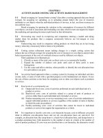
19-16 (30 min.) Costs of quality.
1.

The ratios of each COQ category to revenues and to total quality costs for each period are as follows:
Costen, Inc.: Semi-annual Costs of Quality Report
(in thousands)
6/30/2010

12/31/2010

6/30/2011

12/31/2011

% of Total
% of Total
% of Total
% of Total
% of
Quality
% of
Quality

% of
Quality
% of
Quality
Actual Revenues
Costs
Actual Revenues
Costs
Actual Revenues
Costs
Actual Revenues
Costs
(2) =
(3) =
(5) =
(6) =
(8) =
(9) =
(11) =
(12) =
(1) (1) ÷ $8,240 (1) ÷ $2,040 (4) (4) ÷ $9,080 (4) ÷ $2,159 (7) (7) ÷ $9,300 (7) ÷ $1,605 (10) (10) ÷ $9,020 (10) ÷ $1,271
Prevention costs
Machine maintenance
Supplier training
Design reviews
Total prevention costs
Appraisal costs
Incoming inspection
Final testing
Total appraisal costs

Internal failure costs
Rework
Scrap
Total internal failure costs
External failure costs
Warranty repairs
Customer returns
Total external failure costs
Total quality costs
Total production and revenues

$ 440
20
50
510
108
332
440
231
124
355
165
570
735
$2,040
$8,240

6.2%

5.3%

4.3%

8.9%
24.7%

25.0%

$ 440
100
214
754

21.6%

123
332
455

17.4%

202
116
318

36.0%
100.0%

19-4

85
547
632
$2,159
$9,080

8.3%

5.0%

3.5%

7.0%
23.8%

34.9%

$ 390
50
210
650

21.1%

90
293
383

14.7%

165
71
236

29.3%
100.0%

72
264
336
$1,605
$9,300

7.0%

4.1%

2.5%

3.6%
17.2%

40.5%

$ 330
40
200
570

6.3%

44.9%

23.9%

63
203
266

3.0%

20.9%

14.7%

112
67
179

2.0%

14.1%

2.8%
14.1%

20.1%
100.0%

20.9%

100.0%

68
188
256
$1,271
$9,020


To download more slides, ebook, solutions and test bank, visit

2.
From an analysis of the Cost of Quality Report, it would appear that Costen, Inc.’s
program has been successful because:
Total quality costs as a percentage of total revenues have declined from 24.7% to
14.1%.
External failure costs, those costs signaling customer dissatisfaction, have declined
from 8.9% of total revenues to 2.8% of total revenues and from 36% of all quality
costs to 20.1% of all quality costs. These declines in warranty repairs and customer
returns should translate into increased revenues in the future.
Internal failure costs as a percentage of revenues have been halved from 4.3% to 2%.
Appraisal costs have decreased from 5.3% to 3% of revenues. Preventing defects
from occurring in the first place is reducing the demand for final testing.
Quality costs have shifted to the area of prevention where problems are solved before
production starts: total prevention costs (maintenance, supplier training, and design
reviews) have risen from 25% to 44.9% of total quality costs. The $60,000 increase in
these costs is more than offset by decreases in other quality costs.
Because of improved designs, quality training, and additional pre-production
inspections, scrap and rework costs have almost been halved while increasing sales
by 9.5%.

Production does not have to spend an inordinate amount of time with customer
service since they are now making the product right the first time and warranty
repairs and customer returns have decreased.
3.
To estimate the opportunity cost of not implementing the quality program and to help her
make her case, Jessica Tolmy could have assumed that:
Sales and market share would continue to decline if the quality program was not
implemented and then calculated the loss in revenue and contribution margin.
The company would have to compete on price rather than quality and calculated the
impact of having to lower product prices.
Opportunity costs are not recorded in accounting systems because they represent the results of
what might have happened if the company had not improved quality. Nevertheless, opportunity
costs of poor quality can be significant. It is important for Costen to take these costs into account
when making decisions about quality.

19-5


To download more slides, ebook, solutions and test bank, visit

19-17 (20 min.) Costs of quality analysis.
1.

Appraisal cost = Inspection cost
= $4 × 250,000 car seats
= $1,000,000

2.

Internal failure cost = Rework cost

= 9% × 250,000 × $0.75
= 22,500 × $0.75 = $16,875

3.

Out of pocket external failure cost = Shipping cost + Repair cost
= 3% × 250,000 × ($7 + $0.75)
= 7,500 × $7.75 = $58,125

4.

Opportunity cost of external failure = Lost future profits
= (3% × 250,000) × 20% × $300
= 1,500 car seats × $300 = $450,000

5.

Total cost of quality control = $1,000,000 + $16,875 + $58,125 + $450,000
= $1,525,000

6.

Quality control costs under the alternative inspection technique:
Appraisal cost = $1 × 250,000 = $250,000
Internal failure cost = 5% × 250,000 × $0.75 = $9,375
Out-of-pocket external failure cost = 7% × 250,000 × ($7 + $0.75)
= 17,500 × $7.75 = $135,625
Opportunity cost of external failure = 17,500 car seats × 20% × $300
= 3,500 car seats × $300 = $1,050,000
Total cost of quality control = $250,000 + $9,375 + $135,625 + $1,050,000

= $1,445,000

7.
In addition to the lower costs under the alternative inspection plan, Safe Rider should
consider a number of other factors:
a. There could easily be serious reputation effects if the percentage of external failures
increases by 133% (from 3% to 7%). This rise in external failures may lead to costs
greater than $300 per failure due to lost profits.
b. Higher external failure rates may increase the probability of lawsuits.
c. Government intervention is a concern, with the chances of government regulation
increasing with the number of external failures.

19-6


To download more slides, ebook, solutions and test bank, visit

19-18 (15 min.) Cost of quality analysis, ethical considerations (continuation of 19-17).
1. Cost of improving quality of plastic = $15 × 250,000 = $3,750,000
2. Total cost of lawsuits = 3 × $775,000 = $2,325,000
3. While economically this may seem like a good decision, qualitative factors should be more
important than quantitative factors when it comes to protecting customers from harm and
injury. If a product can cause a customer serious harm and injury, an ethical and moral
company should take steps to prevent that harm and injury. The company’s code of ethics
should guide this decision.
4. In addition to ethical considerations, the company should consider the societal cost of this
decision, reputation effects if word of these problems leaks out at a later date, and
governmental intervention and regulation.

19-7

To download more slides, ebook, solutions and test bank, visit

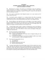
19-19 (25 min.)

Nonfinancial measures of quality and time.

1.

2010
100
= 5%
2,000

2011
400
= 4%
10,000

150
= 7.5%
2,000

250
= 2.5%
10,000

Percentage of units reworked
during production

120
= 6%
2,000

700
= 7%
10,000

Manufacturing cycle time as a
percentage of total time from
order to delivery

15 days
= 50%
30 days

16 days
= 57%
28 days

Percentage of defective units
shipped
Customer complaints as a
percentage of units shipped

2.
Quality has by and large improved. The percentage of defects has decreased by 1
percentage point and the number of customer complaints has decreased by 5 percentage points.
The former indicates an increase in the quality of the cell phones being produced. The latter has

positive implications for future sales. However, the percentage of units reworked has also
increased. WCP should look into the reason for the increase. One possible explanation is the
five-fold increase in production that may have resulted in a higher percentage of errors. WCP
should do a root-cause analysis to identify reasons for the additional rework. Finally, the average
time from order placement to order delivery has decreased. So customers are receiving their
orders on a timelier basis. But manufacturing cycle time is a higher fraction of customer
response time. WCP should seek ways to reduce manufacturing cycle time. For example,
process improvements could reduce both rework and manufacturing cycle time. Any reduction
in manufacturing cycle time would help to further reduce customer response time.
3.
Manufacturing cycle time = wait time + manufacturing time. Producing 10,000 cell
phones in 2011 may have required more waiting time for each order than the waiting time from
producing 2,000 cell phones in 2010. Manufacturing cycle time may have increased as more
time was spent on making products with fewer defects and reducing rework activities.
Customer response time = receipt time + manufacturing cycle time + delivery time.
Manufacturing cycle time is a subset of customer response time. Lower customer response time
times is due to order processing efficiency and/or delivery efficiency and not manufacturing
cycle time.

19-8


To download more slides, ebook, solutions and test bank, visit

19-20 (25 min.) Quality improvement, relevant costs, and relevant revenues.
1.

Relevant costs over the next year of changing to the new component
= $70 18,000 copiers = $1,260,000
Relevant Benefits over

the Next Year of Choosing
the New Component
Costs of quality items
Savings in rework costs
$79 14,000 rework hours
Savings in customer-support costs
$35 850 customer-support hours
Savings in transportation costs for parts
$350 225 fewer loads
Savings in warranty repair costs
$89 8,000 repair-hours
Opportunity costs
Contribution margin from increased sales
Cost savings and additional contribution margin

$1,106,000
29,750
78,750
712,000
1,680,000
$3,606,500

Because the expected relevant benefits of $3,606,500 exceed the expected relevant costs of the
new component of $1,260,000, SpeedPrint should introduce the new component. Note that the
opportunity cost benefits in the form of higher contribution margin from increased sales is an
important component for justifying the investment in the new component.
2.
The incremental cost of the new component of $1,260,000 is less than the incremental
savings in rework and repair costs of $1,926,500 ($1,106,000 + $29,750 + $78,750 + $712,000).
Thus, it is beneficial for SpeedPrint to invest in the new component even without making any

additional sales.

19-9


To download more slides, ebook, solutions and test bank, visit

19-21 (20 min.) Quality improvement, relevant costs, relevant revenues.
1.
Budgeted variable cost per attendee:
Customer support and service personnel
Food and drink
Conference materials
Incidental products and services
Total budgeted variable cost per attendee
Total budgeted variable cost ($205 × 50,000 attendees)
Budgeted fixed costs:
Building and facilities
Management salaries
Total budgeted fixed costs
Total budgeted costs
Budgeted operating income
Budgeted revenues
Budgeted revenue per conference attendee
($18,750,000 ÷ 50,000)

$ 55
100
35
15

$205
$10,250,000
$3,600,000
1,400,000
5,000,000
15,250,000
3,500,000
$18,750,000
$375

The budgeted revenue per conference attendee is $375.
2. Quality improvements: additional menu items; additional incidental products and services;
improved facilities.
Budgeted variable cost per attendee:
Customer support and service personnel ($55 + $3)
Food and drink ($100 + $5)
Conference materials ($35 + $0)
Incidental products and services ($15 + $2)
Total budgeted variable cost per attendee
Budgeted revenues ($375 per attendee 70,000 attendees)
Total budgeted variable costs ($215 70,000 attendees)
Budgeted fixed costs:
Building and facilities (3,500,000 1.50)
Management salaries (1,500,000 1.50)
Total budgeted fixed costs
Total budgeted costs
Budgeted operating income`

19-10

$ 58
105
35
17
$215
$26,250,000
15,050,000
$5,250,000
2,250,000
7,500,000
22,550,000
$ 3,700,000


To download more slides, ebook, solutions and test bank, visit

The improvements above would increase operating income from $3,500,000 to $3,700,000.
Moreover, improving the company’s meeting facilities could also lead to long-term growth.
3. Using information from requirement 2,
Revenues
Fixed costs
Denote total variable costs by $x
$26,250,000 – $x – $7,500,000 = $3,500,000
$x = $26,250,000 – $7,500,000 – $3,500,000
= $15,250,000
Total variable costs = $15,250,000

$26,250,000
$7,500,000

$15, 250, 000
= $217.86
70, 000
At a variable cost per conference attendee of $217.86, Flagstar would be indifferent between
implementing and not implementing the proposed changes.

Variable cost per conference attendee =

19-11


To download more slides, ebook, solutions and test bank, visit

19-22 (30 min.)

Waiting time, service industry.

1. If SMU’s advisors expect to see 300 students each day and it takes an average of 12 minutes to
advise each student, then the average time that a student will wait can be calculated using the
following formula:
2
Average number
Time taken to
advise a student
of students per day
Wait time =
Maximum amount
Average number
Time taken to
2

advise
a student
of students per day
of time available
=

=

300

12

10 hours

2

2

10 advisors

60 minutes

2

43,200
= 9 minutes
6, 000 3, 600

300 12

2. At 420 students seen a day,

Average number
of students per day

Wait time =

Average amount
of students per day

Maximum amount
of time available

2

420

=

=

Time taken to
advise a student

Time taken to
advise a student

2

12

10 hours

2

2

10 advisors

60 minutes

2

60,480
= 31.5 minutes
6, 000 5,040

420 12

3. If the average time to advise a student is reduced to 10 minutes, then the average wait time
would be
2
Average number
Time taken to
advise a student
of students per day
=

2
=

=

Average amount
of students per day

Maximum amount
of time available
420

2

10 advisors

2

42,000
6, 000 4, 200

10 hours

10

2

60 minutes

11.67 minutes

19-12

420 10

Time taken to
advise a student


To download more slides, ebook, solutions and test bank, visit

19-23 (25 min.) Waiting time, cost considerations, and customer satisfaction
(continued from 19-24).
1.

i)

If SMU hires two more advisors then the average wait time will be:

Average number
of students per day

=

=

420
2

Average amount
of students per day

Maximum amount
of time available

2

12 advisors
=

2

Time taken to
advise a student

12

10 hours

2

Time taken to
advise a student

2

60 minutes

420 12

60,480
= 14 minutes

7, 200 5, 040

ii) If SMU has its current employees work 6 days a week and has them advise 350
students a day then the average wait time will be:

Average number
of students per day

=

Maximum amount
of time available

2

=

350
2

10 advisors
=

2

Average amount
of students per day
12

10 hours

50,400
6, 000 4, 200

Time taken to
advise a student

2

Time taken to
advise a student

2

60 minutes

350 12

14 minutes

2. i) Cost if SMU hires 2 extra advisors for the registration period:
Advisor salary cost = 12 advisors ×10 days × $100 = $12,000
ii) Cost if SMU has its 10 advisors work 6 days a week for the registration period:
Advisor salary cost = 10 advisors × 10 days × $100 + 10 advisors × 2 days ×
$150 = $13,000
Alternative (i) is less costly for SMU.
3. Hiring two extra advisors has the same waiting time and a lower cost than extending the
workweek to 6 days during the registration period. However, the quality of the advising may not
be as high. The temporary advisors may not be as familiar with the requirements of the
university. They may also be unaware of how to work within the system (i.e., they may not be

aware of alternatives that may be available to help students). Therefore, from a student
satisfaction standpoint, it would be better to have the regular advisors work an extra day in the
week and pay them overtime. This will be more costly for SMU but is likely to result in better
student advising.
19-13


To download more slides, ebook, solutions and test bank, visit

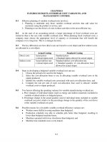
19-24 (15 min.) Manufacturing cycle time, manufacturing cycle efficiency, non-financial
measures of quality.
1, Manufacturing cycle time = Total time from receipt of an order by production until its completion.
Manufacturing cycle time for 2010 = (8 + 6 + 2 + 4 + 2) days = 22 days
Manufacturing cycle time for 2011 = (6 + 7 + 1 + 4 + 2) days = 20 days
Manufacturing cycle efficiency (MCE) is defined as follows:
MCE = Value-added manufacturing time ÷ Manufacturing cycle time
MCE for Torrance Manufacturing for 2010 is:
MCE = 4 days of processing time ÷ 22 days manufacturing cycle time = 0.18
MCE for Torrance Manufacturing for 2011 is:
MCE = 4 days of processing time ÷ 20 days manufacturing cycle time = 0.20
Torrance has become more efficient in its value-added manufacturing time as a percentage of
total manufacturing time during the last year.
Torrance has also shortened its lead time, which means that customers had less time to wait
between placing their order and receiving their shipment. This improvement in timeliness will
likely lead to greater customer satisfaction.
2.
Non-Financial Quality Measure
Percentage of goods returned (as a percentage of units shipped)
(385 14,240; 462 16,834)
Defective units reworked as a percentage of units shipped

(1,122 14,240; 834 16,834)
Percentage of on-time deliveries
(12,438 14,240; 14,990 16,834)
Percentage of hours spent by each employee on quality training
(32 2,000; 36 2,000)

19-14

2010

2011

2.70%

2.74%

7.88%

4.95%

87.35%

89.05%

1.60%

1.80%


To download more slides, ebook, solutions and test bank, visit

3.

Torrance has become more efficient in its value-added manufacturing time as a percentage
of manufacturing cycle time and has improved the company’s lead time. This improved
efficiency should result in cost savings for the company as well as greater customer
satisfaction.
It is important to evaluate the other non-financial quality measures in relation to annual
totals (total units shipped, etc.) rather than as absolute values. For example, the total
number of on-time deliveries increased from 12,438 to 14,990 during 2011. This is an
improvement in the timeliness of the company’s deliveries. As a percentage of total units
delivered, the percentage of on-time deliveries increased from 87.35% to 89.05%.

Management also had two noteworthy areas of improvement related to the non-financial quality
measures above. The first is the reduction in the total number of defective units reworked. This
is a significant improvement over the prior year. However, it should be noted that a greater
percentage of goods were returned in 2011 than in 2010. It is worth further investigation to
analyze if the reduction in rework lead to more defective units being shipped to the end
consumer. Secondly, the company spent an increased amount of time per employee on quality
training. Because quality training programs are considered lead measures of performance, it is
likely that the company will see improvements in the quality of its output in the future due to
improved employee training.

19-15


To download more slides, ebook, solutions and test bank, visit

19-25 (25 min.) Theory of constraints, throughput contribution, relevant costs.
1.

Finishing is a bottleneck operation. Therefore, producing 1,000 more units will generate
additional throughput margin and operating income.
Increase in throughput margin ($72 – $32) 1,000
Incremental costs of the jigs and tools
Increase in operating income investing in jigs and tools

$40,000
30,000
$10,000

Mayfield should invest in the modern jigs and tools because the benefit of higher throughput
margin of $40,000 exceeds the cost of $30,000.
2.
The Machining Department has excess capacity and is not a bottleneck operation.
Increasing its capacity further will not increase throughput margin. There is, therefore, no
benefit from spending $5,000 to increase the Machining Department's capacity by 10,000 units.
Mayfield should not implement the change to do setups faster.
3.
Finishing is a bottleneck operation. Therefore, getting an outside contractor to produce
12,000 units will increase throughput margin.
Increase in throughput margin ($72 – $32) 12,000
Incremental contracting costs $10 12,000
Increase in operating income by contracting 12,000 units of finishing

$480,000
120,000
$360,000

Mayfield should contract with an outside contractor to do 12,000 units of finishing at $10 per
unit because the benefit of higher throughput margin of $480,000 exceeds the cost of $120,000.

The fact that the cost of $10 per unit is double Mayfield's finishing cost of $5 per unit is
irrelevant.
4.
Operating costs in the Machining Department of $640,000, or $8 per unit, are fixed costs.
Mayfield will not save any of these costs by subcontracting machining of 4,000 units to Hunt
Corporation. Total costs will be greater by $16,000 ($4 per unit
4,000 units) under the
subcontracting alternative. Machining more filing cabinets will not increase throughput margin,
which is constrained by the finishing capacity. Mayfield should not accept Hunt's offer. The fact
that Hunt's costs of machining per unit are half of what it costs Mayfield in-house is irrelevant.

19-16


To download more slides, ebook, solutions and test bank, visit

19-26 (15 min.) Theory of constraints, throughput contribution, quality.
1.
Cost of defective unit at machining operation which is not a bottleneck operation is the
loss in direct materials (variable costs) of $32 per unit. Producing 2,000 units of defectives does
not result in loss of throughput margin. Despite the defective production, machining can produce
and transfer 80,000 units to finishing. Therefore, cost of 2,000 defective units at the machining
operation is $32 2,000 = $64,000.
2.
A defective unit produced at the bottleneck finishing operation costs Mayfield materials
costs plus the opportunity cost of lost throughput margin. Bottleneck capacity not wasted in
producing defective units could be used to generate additional sales and throughput margin.
Cost of 2,000 defective units at the finishing operation is:
Loss of direct materials $32 2,000
Forgone throughput margin ($72 – $32)

Total cost of 2,000 defective units

2,000

$ 64,000
80,000
$144,000

Alternatively, the cost of 2,000 defective units at the finishing operation can be calculated as the
lost revenue of $72 2,000 = $144,000. This line of reasoning takes the position that direct
materials costs of $32 2,000 = $64,000 and all fixed operating costs in the machining and
finishing operations would be incurred anyway whether a defective or good unit is produced.
The cost of producing a defective unit is the revenue lost of $144,000.

19-17


To download more slides, ebook, solutions and test bank, visit

19-27 (30 min.) Quality improvement, relevant costs, and relevant revenues.
One way to present the alternatives is via a decision tree, as shown below.
Make T971
Implement
new design

Do not make T971

Do not implement
new design

The idea is to first evaluate the best action that Thomas should take if it implements the
new design (that is, make or not make T971). Thomas can then compare the best mix of products
to produce if it implements the new design against the status quo of not implementing the new
design.
1.
Thomas has capacity constraints. Demand for V262 valves (370,000 valves) exceeds
production capacity of 330,000 valves (3 valves per hour
110,000 machine-hours). Since
capacity is constrained, Thomas will choose to sell the product that maximizes contribution
margin per machine-hour (the constrained resource).
Contribution margin per =
$8 per valve
machine-hour for V262
Contribution margin per =
$10 per valve
machine-hour for T971

3 valves per hour = $24
2 valves per hour = $20.

Thomas should reject Jackson Corporation’s offer and continue to manufacture only
V262 valves.

19-18


To download more slides, ebook, solutions and test bank, visit

2.
Now compare the alternatives of (a) not implementing the new design versus

(b) implementing the new design. By implementing the new design, Thomas will save 10,000
machine-hours of rework time. This time can then be used to make and sell 30,000 (3 valves per
hour 10,000 hours) additional V262 valves. The relevant costs and benefits of implementing
the new design follow:
The relevant costs of implementing the new design

$(315,000)

Relevant benefits:
a
(a) Savings in rework costs ($3 per V262 valve 30,000 valves)
(b) Additional contribution margin from selling another
30,000 V262 valves (3 valves per hour 10,000 hours)
because capacity previously used for rework is freed up
($8 per valve 30,000 units)
Net relevant benefit

90,000

240,000
$

15,000

a

Note that the fixed rework costs of equipment rent and allocated overhead are irrelevant, because these costs
will be incurred whether Thomas implements or does not implement the new design .

Thomas should implement the new design since the relevant benefits exceed the relevant

costs by $15,000.
3.
Thomas Corporation should also consider other benefits of improving quality. For
example, the process of quality improvement will help Thomas's managers and workers gain
expertise about the product and the manufacturing process that may lead to further cost
reductions in the future. Improving quality within the plant is also likely to translate into
delivering better quality products to customers. The increased reputation and customer goodwill
may well lead to higher future revenues through greater unit sales and higher sales prices.

19-19


To download more slides, ebook, solutions and test bank, visit

19-28 (30 min.) Quality improvement, relevant costs, and relevant revenues.
1.
By implementing the new method, Tan would incur additional direct materials costs on all
the 200,000 units started at the molding operation.
Additional direct materials costs = $4 per lamp 200,000 lamps
The relevant benefits of adding the new material are:
Increased revenue from selling 30,000 more lamps
$40 per lamp 30,000 lamps

$800,000

$1,200,000

Note that Tan Corporation continues to incur the same total variable costs of direct
materials, direct manufacturing labor, setup labor and materials handling labor, and the same
fixed costs of equipment, rent, and allocated overhead that it is currently incurring, even when it

improves quality. Since these costs do not differ among the alternatives of adding the new
material or not adding the new material, they are excluded from the analysis. The relevant
benefit of adding the new material is the extra revenue that Tan would get from producing
30,000 good lamps.
An alternative approach to analyzing the problem is to focus on scrap costs and the
benefits of reducing scrap.
The relevant benefits of adding the new material are:
a. Cost savings from eliminating scrap:
Variable cost per lamp, $19a 30,000 lamps
b. Additional contribution margin from selling
another 30,000 lamps because 30,000 lamps
will no longer be scrapped:
Unit contribution margin $21b 30,000 lamps
Total benefits to Tan of adding new material to improve quality

$ 570,000

630,000
$1,200,000

a

Note that only the variable scrap costs of $19 per lamp (direct materials, $16 per lamp; direct manufacturing labor, setup
labor, and materials handling labor, $3 per lamp) are relevant because improving quality will save these costs. Fixed
scrap costs of equipment, rent, and other allocated overhead are irrelevant because these costs will be incurred whether
Tan Corporation adds or does not add the new material.
b

Contribution margin per unit
Selling price

Variable costs:
Direct materials costs per lamp
Molding department variable manufacturing costs
per lamp (direct manufacturing labor, setup labor, and
materials handling labor)
Variable costs
Unit contribution margin

$40.00
$16.00

3.00
(19.00)
$21.00

On the basis of quantitative considerations alone, Tan should use the new material.
Relevant benefits of $1,200,000 exceed the relevant costs of $800,000 by $400,000.
2.
Other nonfinancial and qualitative factors that Tan should consider in making a decision
include the effects of quality improvement on:
a.
gaining manufacturing expertise that could lead to further cost reductions in the
future;
b. enhanced reputation and increased customer goodwill which could lead to higher
future revenues through greater unit sales and higher sales prices; and
c.
higher employee morale as a result of higher quality.
19-20

To download more slides, ebook, solutions and test bank, visit

19-29

(30–40 min.) Statistical quality control.

1.
The + 2 rule will trigger a decision to investigate when mean weight per production run
is outside the control limit:
Double Bran Bits:
Honey Wheat Squares:
Sugar King Pops:

Mean + 2
Mean + 2
Mean + 2

= 17.97 + (2 0.28) or 17.41 to 18.53 oz.
= 14 + (2 0.16) or 13.68 to 14.32 oz.
= 16.02 + (2 0.21) or 15.60 to 16.44 oz.

Any weight less than the lower control limit or greater than the upper control limit will trigger an
investigation by management.
The only cereal weights outside the specified
Pops on production runs #6 and #10.
2.

+ 2 control limit were the Sugar King

Solution Exhibit 19-29 presents the SQC charts for each of the three breakfast cereals.

Double Bran Bits had no observations outside the control limits. Each of the production
runs is considered to be in conformance with quality standards. However, there is an apparent
trend from the SQC that the mean of each of the later production runs gets nearer to the lower
control limit. Even though this product has not violated the quality requirements, management
should investigate the trend to learn if there is faulty equipment or flawed processes that are
causing subsequent runs to result in less cereal per box on average.
Honey Wheat Squares also has no observations outside of the control limits. In fact, this
product seems to be following the quality specifications most closely. Also, variations appear
random in nature and no trends are apparent from the SQC that warrant further investigation by
management.
Sugar King Pops has two observations outside the control limits. One falls below the lower
control limit and one above the upper control limit. These two production runs would not be in
conformance with quality standards. The wide fluctuation in weight variances should be
investigated further by management to determine the failure to comply with quality standards.

19-21


To download more slides, ebook, solutions and test bank, visit

3.

The costs of quality include
(1) Prevention costs—Costs of designing the process, maintaining equipment, and
employee training to operate the production line.
(2) Appraisal costs—Costs of inspection to check the weight of cereal boxes.
(3) Internal failure costs—Costs of refilling cereal boxes that do not meet specifications;
costs to identify causes of failure such as machine calibration, material variability, or
human error; costs of reconfiguring manufacturing processes to prevent errors in

filling cereal boxes.
(4) External failure costs—Costs of customer ill-will if they discover that cereal boxes
are underfilled, costs of returning and replacing incorrectly filled boxes.

Six sigma quality is a standard of excellence that requires a strict understanding of both
customer expectations and reasons for manufacturing defects to improve current quality
performance. The statistical term six sigma translates to 3.4 defects per 1 million incidents, or
near perfection in quality variability. Key aspects of Six Sigma are to Define, Measure, Analyze,
Improve and Control processes. Keltrex Cereals could employ Six Sigma programs to reduce
variability in box weights. The company would first need to 1) define the quality problem (i.e.
variability in weight per cereal box) 2) measure the incidents of defect using statistical quality
control tools 3) analyze potential reasons for variability in the weight per cereal box (machine
calibration, material variability, human error, etc.) 4) Assuming the variability is due to machines
the company may choose to better calibrate the existing machines, purchase new machines that
are more precise, or investigate other engineering alternatives 5) Finally, once improvements
have been made to the existing machines, the company needs to monitor the improvements to
ensure that the variability problem has been resolved.

19-22


To download more slides, ebook, solutions and test bank, visit

SOLUTION EXHIBIT 19-29
Plots of Mean Weight per Production Run for Keltrex Cereals

Weight

Double Bran Bits
18.56

18.42
18.28
18.14
18.00
17.86
17.72
17.58
17.44
17.30

Mean + 2

Mean – 2
0

1

2

3

4

5

6

7

8

9

10

9

10

9

10

Production Run

Weight

Honey Wheat Squares
14.32
14.24
14.16
14.08
14.00
13.92
13.84
13.76
13.68
13.60

Mean+2

Mean–2
0

1

2

3

4

5

6

7

8

Production Run

Weight

Sugar King Pops
16.70
16.56
16.42
16.28
16.14

16.00
15.86
15.72
15.58
15.44

Mean–2

Mean–2
0

1

2

3

4

5

6

Production Run

19-23

7

8

To download more slides, ebook, solutions and test bank, visit

19-30 (30–40 min.) Compensation linked with profitability, waiting time, and quality
measures.
1.
Philadelphia
Add: Profitability
0.75% of operating income
Add: Average waiting time
$40,000 if < 10 minutes
Deduct: Patient satisfaction
$40,000 if < 65
Total: Bonus paid

Jan.-June

Baltimore
Add: Profitability
0.75% of operating income
Add: Average waiting time
$40,000 if < 10 minutes
Deduct: Patient satisfaction
$40,000 if < 65
Total: Bonus paid
2.

July-Dec.

$83,625

$78,750

0

0

0
$83,625

0
$78,750

$71,250

$44,063

0

40,000

(40,000)
$31,250

0
$84,063

Operating income as a measure of profitability

Operating income captures revenue and cost-related factors. However, there is no recognition of
investment differences between the two groups. If one group is substantially bigger than the
other, differences in size alone give the president of the larger group the opportunity to earn a
bigger bonus. An alternative approach would be to use return on investment (perhaps relative to
the budgeted ROI).
10 minute benchmark as a measure of patient response time
This measure reflects the ability of East Coast Healthcare to meet a benchmark for patient
response time. Several concerns arise with this specific measure:
a. It is a yes-or-no cut-off. A 12-minute waiting time earns no bonus, but neither does a
two hour wait. Moreover, no extra bonus is paid for additional waiting time
reductions below 10 minutes. An alternative is to have the bonus that increases with
greater waiting time improvements.
b. It can be manipulated. Doctors might quickly make initial contact with a patient to
meet the benchmark, but then leave the patient sitting in the examination room for a
more detailed examination or procedure to take place.
c. It reflects performance relative only to the initial waiting time. It does not consider
other time-related issues such as the wait for an appointment or the time needed to fill
out forms.

19-24


To download more slides, ebook, solutions and test bank, visit

Problems in (b) and (c) can be overcome by measuring total patient response time (such as how
long it takes from the time a patient makes an appointment to the time the actual appointment is
concluded), in addition to average waiting time to meet the doctor.
Patient satisfaction as a measure of quality
This measure represents a common method for assessing quality. However, there are several
concerns with its use:

a. Patient satisfaction is likely to be influenced by a number of factors that are outside
the groups’ control, such as how sick the patients are when coming in or the extent to
which they follow doctors’ orders.
b. It is influenced by the questions asked in the survey and the survey methodology. As
a result, is likely to be ―noisy‖ or very sensitive to assumptions.
c. Patient satisfaction is not the same as patient health outcomes, an important measure
of healthcare quality.
A combination of measures may work well as a composite measure of quality.
3.
Most companies use both financial and nonfinancial measures to evaluate performance,
sometimes presented in a single report such as a balanced scorecard. Using multiple measures of
performance enables top management to evaluate whether lower-level managers have improved
one area at the expense of others. For example, did the better average waiting time (and patient
satisfaction) between July and December in the Baltimore group result from significantly higher
expenditures that contributed to the dramatic reduction in operating income?
An important issue is the relative importance to place on the different measures. If waiting time
is not used for performance evaluation, managers will concentrate on increasing operating
income and give less attention to waiting time, even if waiting time has a significant influence on
whether customers choose East Coast Healthcare or another healthcare provider when given the
choice. However, the president of the Baltimore group received a larger bonus in the second half
of the year due in part to lower average waiting time, even though operating profits dropped by
nearly 40%. Companies must understand the relative importance of different financial and
nonfinancial objectives when using multiple measures for performance evaluation.

19-25