Solution manual cost management measuring monitoring and motivating performance 1st by wolcott ch03

To download more slides, ebook, solutions and test bank, visit

Chapter 3
Cost-Volume-Profit Analysis
LEARNING OBJECTIVES
Chapter 3 addresses the following questions:
Q1
Q2
Q3
Q4
Q5
Q6

What is cost-volume-profit (CVP) analysis, and how is it used for decision making?
How are CVP calculations performed for a single product?
How are CVP calculations performed for multiple products?
What is the breakeven point?
What assumptions and limitations should managers consider when using CVP analysis?
How are margin of safety and operating leverage used to assess operational risk?

These learning questions (Q1 through Q6) are cross-referenced in the textbook to individual
exercises and problems.

COMPLEXITY SYMBOLS
The textbook uses a coding system to identify the complexity of individual requirements in the
exercises and problems.
Questions Having a Single Correct Answer:
No Symbol
This question requires students to recall or apply knowledge as shown in the
textbook.
This question requires students to extend knowledge beyond the applications

e
shown in the textbook.

Open-ended questions are coded according to the skills described in Steps for Better Thinking
(Exhibit 1.10):

Step 1 skills (Identifying)

Step 2 skills (Exploring)

Step 3 skills (Prioritizing)

Step 4 skills (Envisioning)


To download more slides, ebook, solutions and test bank, visit

3-2

Cost Management

QUESTIONS
3.1

A mixed cost function includes both fixed and variable costs. If there are fixed costs in
the cost function, then total costs will increase at a smaller rate than the increase in total
sales volume. If there are variable costs in the cost function, then total costs will increase
with total sales volume. When there is a combination of fixed and variable costs, a 10%
volume increase will increase total costs by less than 10% because only the increase in
variable cost is proportionate to volume; the fixed cost does not change with volume.

3.2

The weighted average contribution margin per unit is calculated only when performing
CVP analysis for multiple products. There are two ways to calculate it:
(1) Calculate the total contribution of all products by subtracting total variable costs from
total revenues. Then calculate the weighted average contribution margin per unit by
dividing the total contribution margin by the total number of units (the sum of units
for all products).
(2) Calculate the sales mix for each product by dividing the number of units sold for that
product by the total number of units sold for all products. Calculate the contribution
margin per unit for each product by subtracting that product’s variable cost from its
revenues and dividing the result by that product’s number of units sold. Then
calculate the weighted average contribution margin per unit by summing the
following computation for all products: Each product’s sales mix percentage times its
contribution margin per unit.

3.3

The firm has only variable costs and no fixed costs. If there were fixed costs, income
would increase by more than 20% when sales increase by 20%.

3.4

None. The firm does not pay income taxes at the breakeven point.

3.5

Assumptions: Fixed costs remain fixed, variable costs per unit or as a percentage of
revenue remain constant, selling prices per unit remain constant, the sales mix remains

constant, and operations are within a relevant range where all of these assumptions are
met. These are very strong assumptions. There is always some variation in fixed costs
because they include costs such as electricity that varies with weather. In addition,
organizations often get or give volume discounts, so variable costs and prices per unit
may change at high volumes. However, results using these assumptions are accurate
enough for general planning and decision making purposes.

3.6

The margin of safety percentage and degree of operating leverage are related as follows.
Margin of Safety Percentage

Degree of Operating Leverage

1
Degree of Operating Leverage

1
Margin of Safety Percentage


To download more slides, ebook, solutions and test bank, visit

Chapter 3: Cost-Volume-Profit Analysis

3-3

As the degree of operating leverage gets larger (a higher proportion of fixed costs), the
margin of safety percentage gets smaller, and vice versa.
3.7

The cost function is assumed to be linear over a relevant range. If there are volume
discounts, the cost function becomes piece-wise linear and the range of operations within
which the organization is performing must be taken into account in CVP analysis. The
level of operations must be matched with the appropriate part of the function. Each piece
can be considered as a separate relevant range, and the estimated level of activity needs to
be matched with the appropriate relevant range. Otherwise, the analysis will either
understate or overstate variable costs.

3.8

Sales mix is the specific proportion of total sales of each type of good or service that is
sold. A simple example was presented in the chapter for an ice cream store. Usually
about 15% of revenue was from beverages and the rest from ice cream products. As the
proportion of specific products sold changes, the contribution margin ratio changes
because the contribution per unit is different for the different products in the sales mix.

3.9

CVP refers to changes in income over the relevant range of activity; as such, it includes
the notion of breakeven. Breakeven is more narrowly constructed; it focuses on only one
outcome—the single point at which total revenue equals total cost.

3.10

By definition, the margin of safety is the difference between expected unit sales and
breakeven unit sales. If expected unit sales are below breakeven unit sales, the margin of
safety will be negative.

3.11

CVP analysis can be used for planning purposes such as budgets, product emphasis,
setting prices, setting activity levels, setting work schedules, purchasing raw materials,
setting levels for discretionary costs such as advertising and research and development. It
can also help with monitoring operations, and analyzing the operating leverage of an
organization.

3.12

To make decisions about advertising costs, accountants predict the amount of cost to be
incurred and predict the increase in sales. CVP analysis is then used to determine
whether the increase in cost is equal to or greater than the increase in contribution margin
from additional units sold.

3.13

Good managers are likely to always ask for sensitivity analysis because uncertainty about
sales volumes and other factors always exists. However, when unanticipated changes in
the business environment or consumer preferences arise, managers will be even more
interested in sensitivity analysis. By analyzing a variety of scenarios, managers can
respond more quickly to unanticipated changes.


To download more slides, ebook, solutions and test bank, visit

3-4

Cost Management

EXERCISES

3.14 Target Profit, Not-For-Profit Breakeven
A. Information is given on a per unit basis, so use the following equation:
profit = (p-v)q – F
$1,000 = ($7 per gift basket – $2 per gift basket)*Q - $5,000
$6,000 = ($5 per gift basket)*Q
Q = $6,000/$5 per gift basket = 1,200 gift baskets
B. This problem is about a not-for-profit organization. Many not-for-profit organizations
provide services or sell products at a loss and use donations or grants to cover the losses.
As students approach problems in this textbook, they should think briefly about the type
of organization in the problem to help them solve it. This problem is a breakeven
problem with a unit cost of $7.64 and unit revenue of $4.64, or a unit contribution margin
(loss) of $(3.00). In a for-profit organization, these numbers would indicate that the
company loses money on each unit it sells. In a not-for-profit, it may be appropriate to
sell services at a loss, as long as another source of funds covers the loss. In this problem,
the clinic receives a grant from the city, so there is ―fixed‖ revenue in addition to the fees
collected.
Taking the grant into account, the breakeven is:
0 = ($4.64 - $7.64)*Q + $460,000 grant - $236,000 fixed cost
0 = $-3*Q +$224,000
Solving for Q:
3Q = $224,000
Q = 74,667 patients


To download more slides, ebook, solutions and test bank, visit

Chapter 3: Cost-Volume-Profit Analysis

3-5

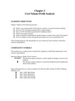
3.15 CVP Graph
A.
CVP Graph 3.15(A)

Total Revenue
Total Cost

$15,000

Dollars

$12,000
$9,000
$6,000
$3,000
$0
0

500

1,000

1,500

2,000

Number of Gift Baskets

The revenue line is $7 times number of baskets and represents total revenue from units
sold. The cost line intersects the intercept at $5,000 reflecting the fixed cost. The slope

is 2, which represents the variable cost. The breakeven occurs at 1,000 gift baskets.
Total revenues exceed total costs by $1,000 at 1,200 gift baskets.
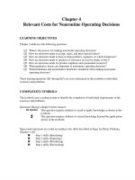
B.
CVP Graph 3.15(B)

Total Revenue
Total Cost

$1,600,000

Dollars

$1,200,000
$800,000
$400,000
$0
0

37,500

75,000 112,500 150,000

Number of Patient Visits

Total revenue is the sum of the grant plus patient fees. Unlike most CVP graphs, the
breakeven point is the maximum volume before the clinic incurs a loss. The grant


To download more slides, ebook, solutions and test bank, visit

3-6

Cost Management
exceeds fixed costs, so the clinic has a surplus up the breakeven point. Because the
clinic’s contribution margin is negative, the surplus decreases by $3 per patient visit.
After the breakeven point of 74,667 patient visits, the clinic incurs losses.

3.16 Cost Function, Breakeven
A. This problem gives information in units, so use the formula TC = v*q + F to determine
variable cost. The average cost must first be turned into total cost:
Total cost for 1,200 units is $234*1,200 = $280,800
Total cost for 1,400 units is $205*1,400 = $287,000
Use the two-point method (change in cost divided by change in volume) to determine the
variable cost:
Variable cost = (287,000 – 280,800)/(1,400 – 1,200)
V = $31
Notice that the information about profit is not used because it is irrelevant for this
problem. Recognizing and discarding irrelevant information is an important skill.
B. Turn sales into units and use profit = (P-V)*Q – F.
Calculate the number of units sold:
Revenue / Selling price per unit = Number of units
$10,600/$0.25 per unit =42,400 units
Variable cost is $0.12 plus selling costs of $0.02 = $0.14 per unit.
Use the breakeven equation, and then solve for the unknown amount of fixed costs:
0 = ($0.25 - $0.14)*42,400 – F
0 = $4,664 – F
F = $4,664
C. There can only be one breakeven point within the relevant range, so the breakeven point
is first calculated for the first range. If the result is within that range, no additional
calculations are needed. However, if the breakeven point is not in the first range, then

calculations must be made for the next range.
In the relevant range 0 < Q < 200, the breakeven point is calculated as:
0 = ($300 - $200)*Q - $24,000
Q = 240 units
This result is outside of the relevant range, so it is not a feasible solution.


To download more slides, ebook, solutions and test bank, visit

Chapter 3: Cost-Volume-Profit Analysis

3-7

In the relevant range 200 < Q, the breakeven point is calculated as:
0 = $100*Q - $36,000
Q = 360 units
This result is in the relevant range, so it is the breakeven point.

3.17 The Martell Company
A. Profit (loss) before taxes is:
$5(1,000,000) - $4.50(1,000,000) -$ 600,000
= $500,000 - $600,000
= $(100,000)
B. Solving for price at target profit of $25,000:
1,000,000*P - $4.50(1,000,000) - $600,000 = $25,000
1,000,000*P = $5,125,000
P = $5.125
The firm needs to have an average selling price of $5.125 to earn $25,000 on sales of
1,000,000 units.
This problem can be used to raise the issue of predatory pricing versus aggressive

competition.

3.18 RainBeau Salon
A.
Cost
Hair dresser salaries
Manicurist salaries
Supplies
Utilities
Rent
Miscellaneous
Total

Fixed
$18,000
16,000
0
400
1,000
2,963
$38,363

Variable

$0.500

0.325
$0.825

TC = $38,363 + $0.825*appointments

Explanations:
Salaries: The amount of salaries in May is used to predict the next month because there
was a cost-of-living increase.


To download more slides, ebook, solutions and test bank, visit

3-8

Cost Management
Supplies: An examination of the pattern in supplies costs reveals that for April and May
supply cost was $0.50 per appointment. The cost was higher in March, but it is best to
use the most current information. Students may have averaged the three months for
$0.52 per month, or they could have used the high-low method which gives $0.50 with no
fixed costs.
Utilities: Because weather probably drives most of utilities cost for this business, this
solution uses the prior month’s utilities to predict next month’s cost.
Miscellaneous: An examination of miscellaneous costs reveals that while it increases as
volumes increase, it does not do so proportionately (as did supplies). For this solution the
high-low method is used. Variable cost = $0.325 [($3,580 - $3,450)/(1,900 – 1,500)].
Using TC = F +VC*Q and solving for F gives a fixed cost of $2,963 [$3,450 = F +
($0.325*1,500)].
B. 0 = ($25.00 - $0.825)Q - $38,363
0 = $24.175*Q - $38,363
Q = 1,587 appointments

3.19 Madden Company
A. Divide sales and variable costs by 160,000 to get the per-unit selling price of $50 and the
variable cost per unit of $12.50.
Then breakeven formula is

$50*Q - $12.50*Q - $3,000,000 = $0
$37.5*Q = $3,000,000
Q = 80,000 units
B. Variable costs are $12.50 per unit/$50.00 per unit = 25% of revenue
Breakeven in sales, where TR = total revenue:
TR - 0.25*TR - $3,000,000 = $4,500,000
0.75*TR= $7,500,000
TR = $10,000,000
C. Target after-tax profit
0.10*$36,000,000 = $3,600,000
After-tax income = (1-0.40)*before tax income


To download more slides, ebook, solutions and test bank, visit

Chapter 3: Cost-Volume-Profit Analysis

3-9

Combining these calculations:
$3,600,000 = 0.60*before tax income
Before-tax income = $6,000,000
CVP calculation:
TR- 0.25*TR - $3,000,000 = $6,000,000
0.75*TR = $9,000,000
TR = $12,000,000

3.20 Laraby Company
A. Selling price per unit
= $625,000/25,000 units= $25/unit

Variable cost per unit
= $375,000/25,000 units= $15/unit
Breakeven point
$25*Q – $15*Q - $150,000 = $0
Q = 15,000 units
B. Adjust the after-tax income target to a before-tax income target.
Income before tax*(1 - .45) = $77,000
Income before tax*0.55 = $77,000
Income before tax = $140,000
Then solve for units at target profit:
$25Q- 15Q - 150,000 = $140,000
Q = 29,000 units
C. Current variable cost
Less old component
Plus new component
New variable cost

$15.00
(2.50)
4.50
$17.00

Solve for breakeven where
$25*Q – $17*Q - $153,000 = $0
Q = 19,125 units

Current fixed cost
Plus depreciation on
new machine $18,000/6
New fixed cost

$150,000
3,000
$153,000


To download more slides, ebook, solutions and test bank, visit

3-10 Cost Management
D. Solve for target profit where:
$25*Q – $17*Q - $153,000 = $100,000 (before tax)
Q = 31,625 units
E. Current contribution margin ratio = ($25 – $15)/$25 = 40%
New price:
P - $17 = 0.40*P
Rearrange terms:
0.60*P = $17
P = $28.33

3.21 Dalton Brothers
A. First determine the pretax income necessary to obtain the $150,000 target net income.
The company is subject to two income tax rates. The first $40,000 of taxable income is
taxed at 15%, and income over that amount is taxed at 40%. Thus, after-tax income is
calculated after subtracting two tax amounts. Assume π = Target pretax income.
π - [0.15 x $40,000 + 0.40*(π - $40,000)] = $150,000
π - (6,000 + 0.4 π - 16,000) = $150,000
0.6 π + 10,000 = $150,000
π = $233,333.33
Now total revenue (TR) can be calculated:
TR - 0.60*TR - $250,000 = $233,333.33

0.40*TR = $483,333.33
TR = $1,208,333.33


To download more slides, ebook, solutions and test bank, visit

Chapter 3: Cost-Volume-Profit Analysis 3-11
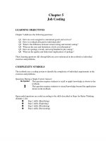
B.

CVP Graph 3.21(B)

Total Revenue
Total Cost

$2,030,000
$1,740,000

Dollars

$1,450,000
$1,160,000
$870,000
$580,000
$290,000
$0
$0

$435,000

$870,000

$1,305,000

$1,740,000

Revenues

3.22 All-Day Candy Company
A. $4*Q - $2.40*Q - $440,000 = $0
Q = 275,000 boxes to break even
B. Current contribution margin ratio = ($4.00-$2.40)/$4.00 = 40%
Estimated variable costs next period (only the candy costs increase)
$2.00 x 1.15 + $0.40 = $2.70
Selling price needed to maintain 40% contribution margin ratio:
P - $2.70 = 0.40*P
0.60*P = $2.70
P = $4.50


To download more slides, ebook, solutions and test bank, visit

3-12 Cost Management
C. Current pretax income = $4.00*390,000 units - $2.40*390,000 units - $440,000
= $184,000
Required sales in units to maintain $184,000 in pretax income:
$4Q - 2.70Q - 440,000 = $184,000
$1.30xQ= $624,000
Q= 480,000 boxes
Dollar sales = 480,000 boxes @ $4 = $1,920,000

3.23 Junior Achievement Group
A. Breakeven for option 1:
$5,600/($20 – $6) = 400 sets
Breakeven for option 2:
New variable cost = 0.10*$20 = $2
$5,600/($20 - $6 - $2) = 317 sets
Breakeven for option 3:
There are no fixed costs, so the breakeven point = 0 sets; if no units are sold, no
fee is paid.
B. The cost function for option 1 has the highest proportion of fixed cost, so it has the
highest operating leverage.
C. Lowest operating risk is option 3 because no fees are paid unless there are sales.
D. To find the indifference point, the two cost equations are set equal to each other as
follows:
$5,600 = $3,800 + 10%TR
$1,800 = 10%TR
TR = $18,000
When total revenues are below $18,000, option 2 is more profitable. Above
$18,000, option 1 is more profitable.


To download more slides, ebook, solutions and test bank, visit

Chapter 3: Cost-Volume-Profit Analysis 3-13
E. Option 1 profit = ($20-$6)*1,000 - $5,600 = $8,400
Option 2 profit = ($20-$6-$2)*1,000 - $3,800 = $8,200
Option 3 profit = ($20-$20*0.15)*1,000= $11,000
The highest profit at sales of 1,000 sets is $11,000 for option 3, so this is probably the
best choice. (This answer ignores possible other factors that might influence the
decision.)

3.24 Borg Controls
A. Expected pretax income:
1,700,000€ - 0.60*1,700,000€ - 321,000€ = 359,000€
Converted to dollars:
359,000€/1.2 € per $= $299,167
ROI = $299,167/$2,680,000 = 11%
B. Target pretax income in dollars:
0.15*$2,680,000 = $402,000
Converted to Euros
$402,000 x 1.2 € per $ = 482,400€
Required revenue
TR - 0.60*TR - 321,000€ = 482,400€
0.40*TR = 803,400
TR = 2,008,500€


To download more slides, ebook, solutions and test bank, visit

3-14 Cost Management
3.25 Newberry’s Nutrition
A. Categorize costs
Cost
Direct materials
Direct labor
Fixed factory overhead
Variable factory overhead
Marketing and Administration
Totals

Fixed

Variable
$300,000
200,000

$100,000
110,000
$210,000

150,000
50,000
$700,000

Variable cost per unit = $700,000/100,000 units = $7.00 per unit
Price per unit = $1,000,000/100,000 units = $10.00 per unit
Target pretax income = $120,000/(1-.40) = $200,000
CVP calculation:
($10.00 - $7.00)Q - $210,000 = $200,000
$410,000 = $3.00*Q
Q = 136,667 units.
B. Before calculating the margin of safety, it is necessary to calculate the breakeven point:
($10.00 - $7.00)Q - $210,000 = $0
Q = $210,000/$3 = 70,000 units
In revenue: 70,000 units * $10 per unit = $700,000
Margin of safety in units
100,000 units – 70,000 units = 30,000 units
Margin of safety in revenues
30,000 units * $10 = $300,000
Double-check computation:

$1,000,000 - $700,000 = $300,000
C. Degree of operating leverage = 1/Margin of safety percentage
= 1/(30,000 units/100,000 units) = 3.33
Double-check calculation:
Degree of operating leverage = (Fixed costs/Expected pretax income) + 1
= ($210,000/$90,000) + 1 = 3.33


To download more slides, ebook, solutions and test bank, visit

Chapter 3: Cost-Volume-Profit Analysis 3-15

3.26 Pike Street Taffy
A. It is first necessary to determine the cost function:
Assuming that the cost of ingredients varies with the amount of taffy produced, the
variable cost per pound is:
$3,200/2,000 lbs = $1.60/lb.
The rent is assumed to be fixed. The wages are also fixed because employees work
standard shifts. Total fixed costs are:
$800+$4800 = $5,600
Breakeven point in pounds:
$5,600/($4.80 per lb. - $1.60 per lb.) = 1,750 lbs.
Breakeven point in revenues:
1,750 lbs * $4.80 per lb. = $8,400
B. Calculate the pretax income needed for an after-tax income of $3,000:
$3,000/(1-20%)=$3,750
Units needed to earn a pretax income of $3,750:
($5,600 + $3,750)/($4.80 per lb. -$1.60 per lb.) = 2,922 lbs.
Revenues needed to earn a pretax income of $3,750:
2,922 lbs * $4.80 per lb. = $14,026

Check calculation using contribution margin ratio formula:
Contribution margin ratio = ($4.80-$1.60)/$4.80 = 66.6667%
($5,600 + $3,750)/66.6667% = $14,025 (difference due to rounding)
C. The margin of safety is current total sales less total sales at breakeven:
=$9,600 - $8,400 = $1,200
The margin of safety percentage = $1,204/$9,600 = 0.125 = 12.5%
(Revenues are 12.5% above the breakeven point)


To download more slides, ebook, solutions and test bank, visit

3-16 Cost Management

D. Degree of operating leverage = contribution margin/pretax income
= ($9,600 - $3,200)/$800 = 8.0
An alternative calculation for degree of operating leverage is:
1/margin of safety percentage
= 1/0.125 = 8.0

3.27 Vines and Daughter
A. Estimated sales in number of swimsuits = $2,000,000/$40 = 50,000 swimsuits
Variable cost per unit = $1,100,000/50,000 swimsuits = $22 per swimsuit
Contribution margin = $40-$22 = $18 per swimsuit
Breakeven in units:
$765,000/$18 = 42,500 swimsuits
B. Margin of safety is 50,000 – 42,500 = 7,500 swimsuits
C. If the margin of safety was 5,000 swimsuits in 2004 and increases to 7,500 swimsuits in
2005 (calculated in Part B), then operations will be less risky in 2005. A larger margin of
safety means that the company is operating further beyond the breakeven point; swimsuit
sales can drop by a larger amount before the company incurs a loss.

D. Contribution margin ratio = $18/$40 = 0.45
Breakeven in revenues:
$765,000/0.45 = $1,700,000
E. Margin of safety in revenue = $2,000,000 - $1,700,000 = $300,000
F. An increase in revenues of $200,000 is expected to increase pretax profits by $90,000 in
profits ($200,000 x 0.45 contribution margin ratio) because fixed costs have been covered
at this point. Total pretax is estimated to be:
$135,000 + $90,000 = $225,000
G. Pretax profit = $180,000/(1-.30) = $257,143
CVP calculation:
($765,000+$257,143)/$18 = 56,786 swimsuits


To download more slides, ebook, solutions and test bank, visit

Chapter 3: Cost-Volume-Profit Analysis 3-17

PROBLEMS
3.28 Oysters Away
[Note about problem complexity: Item A is coded as Extend instead of Step 2 because judgment
is minimal and students can use chapter examples for help.]
A.
Cost
Wages
Packing materials
Rent and Insurance
Admin and selling
Total costs

Fixed

$25,000
45,000
$70,000

Variable
$100,000
20,000

$120,000

Wages are classified as variable because employees are paid an hourly wage and can be
laid off when there is no work. Packing materials would vary with the number of cases
of oysters packed. Rent and insurance are fixed. No information is given about whether
administrative and selling is fixed or variable. It is categorized above as fixed, but it
could be a mixed cost. In the absence of additional information, this solution assumes the
cost is fixed.
Variable cost per case: $120,000/2,000 cases = $60
Cost function: TC = $70,000 + $60*Q
B. Breakeven calculation:
$0 = ($100 - $60)*Q – $70,000
Q = $70,000/$40 per case
Q = 1,750 cases
C. Pretax profit = ($100-$60)*3,000 cases - $70,000
= $120,000 - $70,000 = $50,000
After-tax profit = $50,000 * (1-0.20) = $40,000
D. If only 2,000 cases have been harvested and sold each of the past several years, it is
unlikely that 3,000 cases will be sold next year unless there is some change in operations.
In the absence of information about a change, the quality of the income estimate in Part C
is probably low. In addition, any change in operations major enough to increase sales by

50% might change the cost function (see Part E). So, even if the manager anticipates
expanding the size of operations, the quality of the income estimate is low.
E. It is possible that the costs for workers or packing materials would change above 2,000
cases. If the company does not have enough space to handle all of the oysters, rent would
need to increase. The company might have to pay workers overtime or hire additional


To download more slides, ebook, solutions and test bank, visit

3-18 Cost Management
workers at a higher or lower rate than current workers (depending on skill levels and
supply of workers). With the additional volume, the company might get a discount on
packing materials, so that cost might be smaller. Administrative costs might or might not
increase with the volume of operations. A 50% increase in volume is very significant,
which might require additional administrative costs such as staff, supplies, or fixed
assets.

3.29 Francesca
A.
Quantitative information
Cart lease $800 per month: This is relevant because this is a cost that will be
incurred if Francesca leases the cart, but will not be incurred otherwise.
City license $20 per month: This is relevant for the same reason as the cart
lease.
Lessor records showing average gross revenues of $32 per hour: This
information is relevant if Francesca thinks she will sell about the same
amount as the lessor. However, the lessor’s records might not be
reliable.
Ingredients 40% of revenue: This is relevant because this cost will be incurred
only if Francesca sells coffee.

Last year’s income tax rate of 25%: Assuming that the income tax rate is not
different for operating the coffee cart, the tax rate is irrelevant to
Francesca’s decision. The income tax rate will reduce earnings for both
options.
Condo rent of $1,000 per month and 20% of condo cost for garage: This cost is
not relevant because it will be the same under both options; it is
unavoidable.
Current income $2,400 per month: This is relevant as the opportunity cost if
Francesca decides to operate the coffee cart instead of continuing her
current work.
B. This question calls for calculating the hours Francesca should work to earn a target profit
equal to her current earnings of $2,400 per month. Before this computation can be
performed, the cost function for the coffee cart must be determined:

Cart lease
City license
Ingredients
Total

Fixed
$800
20
$820

Variable

0.40*Revenue
0.40*Revenue

The monthly cost function is estimated as: TC = $820 + 0.40* Revenue

To download more slides, ebook, solutions and test bank, visit

Chapter 3: Cost-Volume-Profit Analysis 3-19
Target profit calculation (assuming that revenue is $32 per hour):
$2,400 = ($32 - 0.40*$32)*Hours per month - $820
$3,220 = $19.2*Hours per month
Hours per month = 168
Assuming that she is willing to work 30 days per month, total hours per month are 168.
Then, the average hours that must be worked per day to earn a target profit of $2,400 is:
168 hours per month/30 days per month = 5.6 hours per day
C. This problem requires students to perform the same calculation as when determining the
selling price needed to achieve a target profit.
Total hours per month = 25 days x 4 hours per day = 100 hours per month
Target profit calculation:
$2,400 = (Revenue per hour - 0.40*Revenue per hour)*100 hours - $820
$3,220 = 60*Revenue per hour
Revenue per hour = $53.67
D. As mentioned in Part A above, Francesca cannot be certain that the information she
received from the lessor is reliable. In addition, revenues are likely to fluctuate based on
weather, the economy, competition, and consumer preferences.
E. There are many other types of information to consider. Some information might help
Francesca evaluate the financial viability of the coffee cart, such as local population
trends, competition, and economic outlook. Additional information relates to Francesca’s
own preferences, such as whether she wants to give up her other occupations and how
much she would enjoy running a coffee cart in Vail.

3.30 Keener Boomerangs
A. Last month 1,200 regular and 2,400 premium boomerangs were sold. Assuming the sales

mix remains constant, two premium boomerangs are sold for each regular boomerang.
B. Total fixed product line costs:
Regular: 1,200 units x $8.17 = $9,804
Premium: 2,400 units x $24.92 = $59,808
C. Total corporate fixed costs: $5.62 x (1,200 + 2,400) units = $20,232


To download more slides, ebook, solutions and test bank, visit

3-20 Cost Management
D. To calculate the overall breakeven, it is easiest to first calculate the weighted average
contribution margin ratio using an income statement approach:
Regular
Premium
Total
Units
1,200
2,400
3,600
Revenue
$26,580
$108,720
$135,300
Variable cost
5,172
16,584
21,756
Contribution margin
$21,408
$ 92,136

$113,544
Weighted average contribution margin ratio ($113,544/$135,300)

83.92%

Overall corporate breakeven (recall that there are three fixed costs):
Revenues = ($9,804 + $59,808 + $20,232)/83.92% = $107,059
Breakeven for Regular based on sales mix in revenues:
$107,059*($26,580/$135,300)
Breakeven for Premium based on sales mix in revenues:
$107,059*($108,720/$135,300)
Total corporate sales at breakeven

$ 21,032

86,027
$107,059

E. Breakeven for regular boomerangs ignoring corporate fixed costs:
Revenues = $9,804/[($22.15-$4.31)/$22.15]
= $9,804/0.8054
= $12,173
F. When regular boomerangs is required to cover only its own fixed costs, the company
does not need to sell as many units to breakeven. The breakeven revenue for boomerangs
is higher when it covers both its own and corporate fixed costs ($21,032) than when it
only covers its own fixed costs ($12,173).
G. Corporate fixed costs are not usually under the control of the individual product
managers. Therefore, corporate fixed costs generally are not considered when evaluating
individual product profitability. However, the company as a whole needs to cover all of
its fixed costs, so it is important to take corporate fixed costs into account when planning

overall operations.
H. The actual sales mix can differ from plans for many reasons. For example, customer
preferences can change, altering the number and prices of units. Competitor’s prices and
products could affect the sales mix. Consumer buying patterns change when the
economy changes. Sometimes an unforeseen event will greatly alter consumer behavior.
These changes cannot easily be predicted.
I. When the sales mix is more uncertain, the quality of information from CVP analysis is
lower because the CVP assumptions are more likely to be violated. Therefore, the
likelihood that the sales mix will remain constant must be evaluated. Sensitivity analysis


To download more slides, ebook, solutions and test bank, visit

Chapter 3: Cost-Volume-Profit Analysis 3-21
should also be performed to examine a larger range of operations that incorporate
possible changes in sales mix. The quality of the CVP analysis is negatively affected by
higher uncertainty about any of the variables used.

3.31 Not-For-Profit After-School Art Program
A.
1. Here are several possible costs; students may think of others.
Cost
Staff people
Art supplies
High school help
Snack food

Category
Fixed (fixed schedule according to # of children)
Mixed, some that will be used up, and some (easels) that

will be fixed
Fixed (fixed schedule according to # of children)
Variable

2. Snack food is the only completely variable cost and number of snacks served would
be a good cost driver. Art supplies have a variable component, and number of
children or number of hours of art would be reasonable cost drivers.
B. The cost structure likely has a larger proportion of fixed costs because salaries for staff
and supervisors would be much higher per hour than the cost of supplies and snacks.
C. The marginal cost is the variable cost (supplies and snacks) per child for three children.
D. The opportunity cost is the revenue foregone from a fee-paying child.
E. CVP analysis offers the neighbor an opportunity to vary assumptions, such as price and
volume of children served while he is considering various options such as scholarships.
A spreadsheet can be set up with an input area for all of the assumptions such as fixed
costs, variable costs, number of children, fees per child, number of fee-paying children,
number of scholarships, and so on. Then the CVP calculations would be performed in a
separate part of the spreadsheet, with cell references to the input cells. The neighbor
could then modify data in the input cells to analyze the expected financial results under
different sets of assumptions.


To download more slides, ebook, solutions and test bank, visit

3-22 Cost Management
3.32 Ersatz
A spreadsheet showing the CVP graph solutions for this problem is available on the Instructor’s
web site for the textbook (available at www.wiley.com/college/eldenburg).
A. The variable cost per unit is the same for 1,000 units and for 1,500 units. Therefore, it is
reasonable to assume that these variable costs will also apply to a volume of 1,300 units.
Variable costs per unit are:

$40 + $10 + $6 = $56 per unit
Fixed costs are:
$10,000 + $11,000 + $20,000 = $41,000
Breakeven is:
$100*Q – $56*Q - $41,000 = $0
Q = 932 units to break even
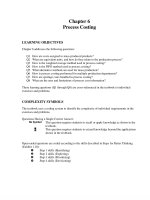
B.
Total Revenue
Total Cost

CVP Graph 3.32(B)

$250,000

Dollars

$200,000
$150,000
$100,000
$50,000
$0
0

500

1,000

1,500

2,000

Number of Units

C. At 1,300 units, pretax income is estimated as:
= ($100 - $56) per unit*1,300 units - $41,000 = $16,200
D. Following is a possible solution to this question. Notice that the message is as short as
possible, yet fully answers the shareholder’s question. The message also avoids use of


To download more slides, ebook, solutions and test bank, visit

Chapter 3: Cost-Volume-Profit Analysis 3-23
highly technical language, but it assumes that the shareholder is familiar with the terms
used in the income statement.
Dear Major Shareholder,
You asked why our profits increased by 800% when sales increased by only 50%.
When we sell 1,000 units, we are very close to the breakeven point—the point at which
our revenues exactly cover our costs. As volume increases above this level, our profit
increases by $44 per unit (our selling price of $100 minus variable costs of $56).
Hence, when sales increase by 500 units, pretax income goes up by $22,000. This will
be true for any 500 unit change in sales. At 1,000 units our pretax income was only
$3,000, so the percentage change when we move from 1,000 units to 1,500 units is
very high.
Please let me know if I can answer any additional questions.
Sincerely,
Accountant
E. New breakeven
$100*(1.03)*Q - $56*(1.03)*Q - $41,000 = $0
$103*Q - $57.68*Q = $41,000
Q= 905 units

The old contribution margin was $44, and the new contribution margin is $45.32, so the
contribution margin per unit has been increased by 3%, causing breakeven unit sales to
decrease.
F. The two approaches will yield the same cost (and, therefore, the same income) when
$11,000 + $10*Q = $20*Q
Q = 1,100 units


To download more slides, ebook, solutions and test bank, visit

3-24 Cost Management
G.

CVP Graph 3.32(G)

Total Revenue
Old Costs

Dollars

New Costs

$250,000
$200,000
$150,000
$100,000
$50,000
$0
0

500

1,000

1,500

2,000

Number of Units

H. If sales exceed 1,100 units, paying $10,000 per period + $10 per unit (the old pay
arrangement) will result in lower total selling costs.
I. Sales representatives with high selling volumes would probably like the new system
because they would be likely to earn more. The opposite would be true for sales
representatives with low selling volumes. Sales representatives who dislike risk might
prefer the existing pay system, which guarantees a minimum payment. People often
dislike any change, so there may be resistance regardless of whether sales representatives
are better off. Overall, the new pay system might encourage sales representatives to
achieve higher sales. It also might lead to higher employee turnover.
J. Pros of changing the system:
Reduces operating risk by reducing fixed costs
Reduces costs if sales are less than 1,100 units
May encourage sales representatives to sell more
Cons of changing the system:
Increases costs if sales are greater than 1,100 units
Could have adverse effects on sales representative morale

3.33 King Salmon Sales
A. This question calls for a breakeven calculation, which means that the cost function must
first be determined. Costs are categorized as shown in the following table. Labor costs

are assumed to be variable because employees work only as needed. Administration cost


To download more slides, ebook, solutions and test bank, visit

Chapter 3: Cost-Volume-Profit Analysis 3-25
is assumed to be fixed because there is no information to suggest that this cost varies
proportionately with volume of activity.
Fixed
Fish
Smoking materials
Packaging materials
Labor
Administration
Sales commission
Total

Variable
$200,000
20,000
30,000
300,000

$150,000
$150,000

10,000
$560,000

If all variable costs vary with pounds of salmon, then variable cost is estimated as:

$560,000/100,000 lbs. = $5.60 per lb.
The cost function is: TC = $150,000 + $5.60 per lb.
If the selling price is the same as last year, it can estimated based on last year’s total
revenue and total volume:
Price = $800,000/100,000 lbs. = $8.00 per lb.
In this problem, it is best to calculate the breakeven in units because there is a limit on the
number of pounds of salmon available:
0 = ($8.00 – $5.60)*Q - $150,000
$150,000 = $2.40*Q
Q = 62,500 lbs
The company cannot cover its fixed costs, because it cannot acquire enough salmon to
break even. Therefore, the company should not operate this year. Note: According to
the information in this question, the company will avoid administrative costs if there is no
salmon production. Therefore, there will be zero profit or loss and the company will be
better off if there is no production.
B. The term ―breakeven‖ has a slightly different meaning in this question than usual. In this
question, ―breakeven‖ means being at least as well off as the alternative. The loss at the
maximum possible production volume of 50,000 lbs. = ($8.00 – $5.60)*50,000 lbs. –
$150,000 = –$30,000. If the company incurs administrative costs whether or not it
produces salmon, then the loss with no production would be –$150,000. Therefore, the
company would be better off producing salmon and incurring a smaller loss.
C. Breakeven price:
0 = (P-$5.60)*50,000 lbs. - $150,000
P = $8.60