Solution manual introduction managerial accounting 5e by garrison chapter 05

To download more slides, ebook, solutions and test bank, visit

Chapter 5
Cost Behavior: Analysis and Use
Solutions to Questions
5-1
a. Variable cost: The variable cost per unit is
constant, but total variable cost changes in
direct proportion to changes in volume.
b. Fixed cost: The total fixed cost is constant
within the relevant range. The average fixed
cost per unit varies inversely with changes
in volume.
c. Mixed cost: A mixed cost contains both
variable and fixed cost elements.
5-2
a. Unit fixed costs decrease as volume
increases.
b. Unit variable costs remain constant as
volume increases.
c. Total fixed costs remain constant as volume
increases.
d. Total variable costs increase as volume
increases.

or decreases in total in direct relation to
changes in activity.
b. Mixed cost: A mixed cost is a cost that
contains both variable and fixed cost
elements.
c. Step-variable cost: A step-variable cost is a

cost that is incurred in large chunks, and
which increases or decreases only in
response to fairly wide changes in activity.

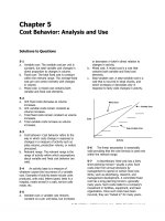
Mixed Cost
Variable Cost

Cost

Step-Variable Cost

5-3
a. Cost behavior: Cost behavior refers to the
way in which costs change in response to
changes in a measure of activity such as
sales volume, production volume, or orders
processed.
b. Relevant range: The relevant range is the
range of activity within which assumptions
about variable and fixed cost behavior are
valid.
5-4
An activity base is a measure of
whatever causes the incurrence of a variable
cost. Examples of activity bases include units
produced, units sold, letters typed, beds in a
hospital, meals served in a cafe, service calls
made, etc.
5-5
a. Variable cost: A variable cost remains

constant on a per unit basis, but increases

Activity

5-6
The linear assumption is reasonably
valid providing that the cost formula is used only
within the relevant range.
5-7
A discretionary fixed cost has a fairly
short planning horizon—usually a year. Such
costs arise from annual decisions by
management to spend on certain fixed cost
items, such as advertising, research, and
management development. A committed fixed
cost has a long planning horizon—generally
many years. Such costs relate to a company’s
investment in facilities, equipment, and basic
organization. Once such costs have been
incurred, they are ―locked in‖ for many years.

© The McGraw-Hill Companies, Inc., 2010. All rights reserved.
Solutions Manual, Chapter 5

199


To download more slides, ebook, solutions and test bank, visit

5-8

a. Committed
b. Discretionary
c. Discretionary

d. Committed
e. Committed
f. Discretionary

5-9
Yes. As the anticipated level of activity
changes, the level of fixed costs needed to
support operations may also change. Most fixed
costs are adjusted upward and downward in
large steps, rather than being absolutely fixed at
one level for all ranges of activity.
5-10 The high-low method uses only two
points to determine a cost formula. These two
points are likely to be less than typical because
they represent extremes of activity.
5-11 The formula for a mixed cost is Y = a +
bX. In cost analysis, the ―a‖ term represents the
fixed cost and the ―b‖ term represents the
variable cost per unit of activity.
5-12 In a least-squares regression, the sum
of the squares of the deviations from the plotted
points on a graph to the regression line is

smaller than could be obtained from any other
line that could be fitted to the data.
5-13 Ordinary single least-squares regression

analysis is used when a variable cost is a
function of only a single factor. If a cost is a
function of more than one factor, multiple
regression analysis should be used to analyze
the behavior of the cost.
5-14 The contribution approach income
statement organizes costs by behavior, first
deducting variable expenses to obtain
contribution margin, and then deducting fixed
expenses to obtain net operating income. The
traditional approach organizes costs by function,
such as production, selling, and administration.
Within a functional area, fixed and variable costs
are intermingled.
5-15 The contribution margin is total sales
revenue less total variable expenses.

© The McGraw-Hill Companies, Inc., 2010. All rights reserved.
200

Introduction to Managerial Accounting, 5th Edition


To download more slides, ebook, solutions and test bank, visit

Brief Exercise 5-1 (15 minutes)
1.
Fixed cost ................................
Variable cost ............................
Total cost ................................

Average cost per cup of coffee
served * ................................

Cups of Coffee Served
in a Week
2,000
2,100
2,200

$1,200
440
$1,640
$0.820

$1,200
462
$1,662
$0.791

$1,200
484
$1,684
$0.765

* Total cost ÷ cups of coffee served in a week
2. The average cost of a cup of coffee declines as the number of cups of
coffee served increases because the fixed cost is spread over more cups
of coffee.

© The McGraw-Hill Companies, Inc., 2010. All rights reserved.

Solutions Manual, Chapter 5

201


To download more slides, ebook, solutions and test bank, visit

Brief Exercise 5-2 (30 minutes)
1. The scattergraph appears below:
$60,000

Y

Processing Cost

$50,000

$40,000

$30,000

$20,000

$10,000

$0
0

2,000

4,000

6,000

X
8,000 10,000 12,000 14,000

Units Produced

© The McGraw-Hill Companies, Inc., 2010. All rights reserved.
202

Introduction to Managerial Accounting, 5th Edition


To download more slides, ebook, solutions and test bank, visit

Brief Exercise 5-2 (continued)
2. (Students’ answers will vary considerably due to the inherent
imprecision of the quick-and-dirty method.)
The approximate monthly fixed cost is $30,000—the point where the
line intersects the cost axis. The variable cost per unit processed can be
estimated using the 8,000-unit level of activity, which falls on the line:
Total cost at an 8,000-unit level of activity ............
Less fixed costs ...................................................
Variable costs at an 8,000-unit level of activity ......

$46,000
30,000
$16,000

$16,000 ÷ 8,000 units = $2 per unit
Therefore, the cost formula is $30,000 per month plus $2 per unit
processed.
Observe from the scattergraph that if the company used the high-low
method to determine the slope of the regression line, the line would be
too steep. This would result in underestimating fixed costs and
overestimating the variable cost per unit.

© The McGraw-Hill Companies, Inc., 2010. All rights reserved.
Solutions Manual, Chapter 5

203


To download more slides, ebook, solutions and test bank, visit

Brief Exercise 5-3 (20 minutes)
1.
High activity level (August) ..
Low activity level (October)..
Change ...............................

OccupancyDays
2,406
124
2,282

Electrical
Costs

$5,148
1,588
$3,560

Variable cost = Change in cost ÷ Change in activity
= $3,560 ÷ 2,282 occupancy-days
= $1.56 per occupancy-day
Total cost (August) ....................................................
Variable cost element
($1.56 per occupancy-day × 2,406 occupancy-days)
Fixed cost element ....................................................

$5,148
3,753
$1,395

2. Electrical costs may reflect seasonal factors other than just the variation
in occupancy days. For example, common areas such as the reception
area must be lighted for longer periods during the winter than in the
summer. This will result in seasonal fluctuations in the fixed electrical
costs.
Additionally, fixed costs will be affected by the number of days in a
month. In other words, costs like the costs of lighting common areas are
variable with respect to the number of days in the month, but are fixed
with respect to how many rooms are occupied during the month.
Other, less systematic, factors may also affect electrical costs such
as the frugality of individual guests. Some guests will turn off lights
when they leave a room. Others will not.

© The McGraw-Hill Companies, Inc., 2010. All rights reserved.

204

Introduction to Managerial Accounting, 5th Edition


To download more slides, ebook, solutions and test bank, visit

Brief Exercise 5-4 (20 minutes)
1.
The Alpine House, Inc.
Income Statement—Ski Department
For the Quarter Ended March 31
Sales ....................................................................
Variable expenses:
Cost of goods sold (200 pairs* × $450 per pair) ...
Selling expenses (200 pairs × $50 per pair) ..........
Administrative expenses (20% × $10,000) ...........
Contribution margin ...............................................
Fixed expenses:
Selling expenses
[$30,000 – (200 pairs × $50 per pair)] ..............
Administrative expenses (80% × $10,000) ...........
Net operating income ............................................

$150,000
$90,000
10,000
2,000

20,000

8,000

102,000
48,000

28,000
$ 20,000

*$150,000 ÷ $750 per pair = 200 pairs
2. Since 200 pairs of skis were sold and the contribution margin totaled
$48,000 for the quarter, the contribution of each pair of skis toward
covering fixed costs and toward earning of profits was $240 ($48,000 ÷
200 pairs = $240 per pair). Another way to compute the $240 is:
Selling price per pair ..........................
Variable expenses:
Cost per pair ...................................
Selling expenses..............................
Administrative expenses
($2,000 ÷ 200 pairs).....................
Contribution margin per pair ...............

$750
$450
50
10

510
$240

© The McGraw-Hill Companies, Inc., 2010. All rights reserved.

Solutions Manual, Chapter 5

205


To download more slides, ebook, solutions and test bank, visit

Exercise 5-5 (20 minutes)
1. The company’s variable cost per unit is:
$180,000
=$6 per unit.
30,000 units

In accordance with the behavior of variable and fixed costs, the
completed schedule is:

Total costs:
Variable costs ............
Fixed costs ................
Total costs .................
Cost per unit:
Variable cost ..............
Fixed cost ..................
Total cost per unit ......

Units produced and sold
30,000
40,000
50,000
$180,000

300,000
$480,000
$ 6.00
10.00
$16.00

$240,000 $300,000
300,000 300,000
$540,000 $600,000
$ 6.00
7.50
$13.50

$ 6.00
6.00
$12.00

2. The company’s income statement in the contribution format is:
Sales (45,000 units × $16 per unit) ........................
Variable expenses (45,000 units × $6 per unit) .......
Contribution margin...............................................
Fixed expense .......................................................
Net operating income ............................................

$720,000
270,000
450,000
300,000
$150,000

© The McGraw-Hill Companies, Inc., 2010. All rights reserved.
206

Introduction to Managerial Accounting, 5th Edition


To download more slides, ebook, solutions and test bank, visit

Exercise 5-6 (45 minutes)
1.

High activity level (June)......
Low activity level (July)........
Change ...............................

Units Shipped Shipping Expense
8
2
6

$2,700
1,200
$1,500

Variable cost element:
Change in expense $1,500
=
=$250 per unit.
Change in activity 6 units

Fixed cost element:
Shipping expense at high activity level .......................
Less variable cost element ($250 per unit × 8 units)...
Total fixed cost .........................................................

$2,700
2,000
$ 700

The cost formula is $700 per month plus $250 per unit shipped or
Y = $700 + $250X,
where X is the number of units shipped.
2. a. See the scattergraph on the following page.
b. (Note: Students’ answers will vary due to the imprecision of this
method of estimating variable and fixed costs.)
Total cost at 5 units shipped per month [a point
falling on the regression line in (a)]......................
Less fixed cost element (intersection of the Y axis)..
Variable cost element.............................................

$2,000
1,000
$1,000

$1,000 ÷ 5 units = $200 per unit
The cost formula is $1,000 per month plus $200 per unit shipped or
Y = $1,000 + $200X
where X is the number of units shipped.

© The McGraw-Hill Companies, Inc., 2010. All rights reserved.

Solutions Manual, Chapter 5

207


To download more slides, ebook, solutions and test bank, visit

Exercise 5-6 (continued)
2. a. The scattergraph would be:
$3,000

Y

Shipping Expense

$2,500
$2,000
$1,500
$1,000
$500
X

$0
0

2

4

6

8

10

Units Shipped

3. The cost of shipping units is likely to depend on the weight and volume
of the units and the distance traveled, as well as on the number of units
shipped. In addition, higher cost shipping might be necessary to meet a
deadline.

© The McGraw-Hill Companies, Inc., 2010. All rights reserved.
208

Introduction to Managerial Accounting, 5th Edition


To download more slides, ebook, solutions and test bank, visit

Exercise 5-7 (20 minutes)
1.
High level of activity .........................
Low level of activity ..........................
Change ............................................

Kilometers Total Annual
Driven
Cost*
105,000

70,000
35,000

$11,970
9,380
$ 2,590

* 105,000 kilometers × $0.114 per kilometer = $11,970
70,000 kilometers × $0.134 per kilometer = $9,380
Variable cost per kilometer:
Change in cost
$2,590
=
=$0.074 per kilometer
Change in activity 35,000 kilometers

Fixed cost per year:
Total cost at 105,000 kilometers .....................
Less variable portion:
105,000 kilometers × $0.074 per kilometer ..
Fixed cost per year ........................................

$11,970
7,770
$ 4,200

2. Y = $4,200 + $0.074X
3. Fixed cost .........................................................
Variable cost:
80,000 kilometers × $0.074 per kilometer ........

Total annual cost ...............................................

$ 4,200
5,920
$10,120

© The McGraw-Hill Companies, Inc., 2010. All rights reserved.
Solutions Manual, Chapter 5

209


To download more slides, ebook, solutions and test bank, visit

Exercise 5-8 (20 minutes)
1.
High activity level (July) ...............
Low activity level (March) ............
Change .......................................

Custodial
Guest- Supplies
Days Expense
12,000
4,000
8,000

$13,500
7,500
$ 6,000

Variable cost element:
Change in expense
$6,000
=
=$0.75 per guest-day
Change in activity 8,000 guest-days

Fixed cost element:
Custodial supplies expense at high activity level ....
Less variable cost element:
12,000 guest-days × $0.75 per guest-day ..........
Total fixed cost ....................................................

$13,500
9,000
$ 4,500

The cost formula is $4,500 per month plus $0.75 per guest-day or
Y = $4,500 + $0.75X
2. Custodial supplies expense for 11,000 guest-days:
Variable cost:
11,000 guest-days × $0.75 per guest-day .
Fixed cost ..................................................
Total cost ...................................................

$ 8,250
4,500
$12,750

© The McGraw-Hill Companies, Inc., 2010. All rights reserved.
210

Introduction to Managerial Accounting, 5th Edition


To download more slides, ebook, solutions and test bank, visit

Exercise 5-9 (30 minutes)
1. The scattergraph appears below:

$16,000

Y

Custodial Supplies Cost

$14,000
$12,000
$10,000
$8,000
$6,000
$4,000
$2,000
X

$0
0

2,000 4,000 6,000 8,000 10,000 12,000 14,000

Guest-Days

© The McGraw-Hill Companies, Inc., 2010. All rights reserved.
Solutions Manual, Chapter 5

211


To download more slides, ebook, solutions and test bank, visit

Exercise 5-9 (continued)
2. (Note: Students’ answers will vary considerably due to the inherent lack
of precision and subjectivity of the quick-and-dirty method.)
Total costs at 7,500 guest-days per month [a point
falling on the line in (1)] .........................................
Less fixed cost element (intersection of the Y axis) .....
Variable cost element ................................................

$9,750
3,750
$6,000

$6,000 ÷ 7,500 guest-days = $0.80 per guest-day
The cost formula is therefore $3,750 per month, plus $0.80 per guestday or
Y = $3,750 + $0.80X,
where X is the number of guest-days.
3. The high-low method would not provide an accurate cost formula in this
situation because a line drawn through the high and low points would
have a slope that is too flat and would be placed too high, cutting the

cost axis at about $4,500 per month. The high and low points are not
representative of all of the data in this situation.

© The McGraw-Hill Companies, Inc., 2010. All rights reserved.
212

Introduction to Managerial Accounting, 5th Edition


To download more slides, ebook, solutions and test bank, visit

Exercise 5-10 (20 minutes)
1. a. Difference in cost:
Monthly operating costs at 80% occupancy:
450 beds × 80% = 360 beds;
360 beds × 30 days × $32 per bed-day ....................
Monthly operating costs at 60% occupancy (given) ......
Difference in cost .......................................................

$345,600
326,700
$ 18,900

Difference in activity:
80% occupancy (450 beds × 80% × 30 days) ..........
60% occupancy (450 beds × 60% × 30 days) ..........
Difference in activity ..................................................

10,800
8,100

2,700

Change in cost
$18,900
=
= $7 per bed-day
Change in activity
2,700 bed-days

b. Monthly operating costs at 80% occupancy (above) .....
Less variable costs:
360 beds × 30 days × $7 per bed-day ......................
Fixed operating costs per month .................................

$345,600
75,600
$270,000

2. 450 beds × 70% = 315 beds occupied:
Fixed costs ................................................................ $270,000
Variable costs: 315 beds × 30 days × $7 per bed-day .
66,150
Total expected costs .................................................. $336,150

© The McGraw-Hill Companies, Inc., 2010. All rights reserved.
Solutions Manual, Chapter 5

213

To download more slides, ebook, solutions and test bank, visit

Problem 5-11A (45 minutes)
1.

Marwick’s Pianos, Inc.
Income Statement
For the Month of August
Sales (40 pianos × $3,125 per piano) ...............
Cost of goods sold
(40 pianos × $2,450 per piano) .....................
Gross margin ..................................................
Selling and administrative expenses:
Selling expenses:
Advertising ................................................
Sales salaries and commissions
[$950 + (8% × $125,000)] ......................
Delivery of pianos
(40 pianos × $30 per piano).....................
Utilities ......................................................
Depreciation of sales facilities .....................
Total selling expenses ...................................
Administrative expenses:
Executive salaries .......................................
Insurance ..................................................
Clerical
[$1,000 + (40 pianos × $20 per piano)] ...
Depreciation of office equipment.................
Total administrative expenses ........................
Total selling and administrative expenses ..........

Net operating income ......................................

$125,000
98,000
27,000
$

700

10,950
1,200
350
800
14,000
2,500
400
1,800
300
5,000

19,000
$ 8,000

© The McGraw-Hill Companies, Inc., 2010. All rights reserved.
214

Introduction to Managerial Accounting, 5th Edition


To download more slides, ebook, solutions and test bank, visit

Problem 5-11A (continued)
2.

Marwick’s Pianos, Inc.
Income Statement
For the Month of August

Sales (40 pianos × $3,125 per piano) .................
Variable expenses:
Cost of goods sold
(40 pianos × $2,450 per piano) ....................
Sales commissions (8% × $125,000) ...............
Delivery of pianos (40 pianos × $30 per piano)
Clerical (40 pianos × $20 per piano) ................
Total variable expenses ......................................
Contribution margin...........................................
Fixed expenses:
Advertising .....................................................
Sales salaries ..................................................
Utilities...........................................................
Depreciation of sales facilities ..........................
Executive salaries ...........................................
Insurance .......................................................
Clerical ...........................................................
Depreciation of office equipment .....................
Total fixed expenses ..........................................
Net operating income ........................................

Total

Per
Piano

98,000
10,000
1,200
800
110,000
15,000

2,450
250
30
20
2,750
$ 375

$125,000

$3,125

700
950
350
800
2,500
400
1,000
300

7,000
$ 8,000

3. Fixed costs remain constant in total but vary on a per unit basis
inversely with changes in the activity level. As the activity level
increases, for example, the fixed costs will decrease on a per unit basis.
Showing fixed costs on a per unit basis on the income statement might
mislead management into thinking that the fixed costs behave in the
same way as the variable costs. That is, management might be misled
into thinking that the per unit fixed costs would be the same regardless
of how many pianos were sold during the month. For this reason, fixed
costs generally are shown only in totals on a contribution format income
statement.
© The McGraw-Hill Companies, Inc., 2010. All rights reserved.
Solutions Manual, Chapter 5

215


To download more slides, ebook, solutions and test bank, visit

Problem 5-12A (45 minutes)
1. Cost of goods sold ...................
Advertising expense ................
Shipping expense ....................
Salaries and commissions ........
Insurance expense ..................
Depreciation expense ..............

Variable

Fixed
Mixed
Mixed
Fixed
Fixed

2. Analysis of the mixed expenses:

High level of activity .....
Low level of activity ......
Change ........................

Salaries and
Commissions
Expense

Shipping
Expense

Units

5,000
4,000
1,000

A$38,000
34,000
A$ 4,000

A$90,000

78,000
A$12,000

Variable cost element:
Variable rate =

Change in cost
Change in activity

Shipping expense:

A$4,000
= A$4 per unit
1,000 units

Salaries and commissions expense:

A$12,000
= A$12 per unit
1,000 units

Fixed cost element:

Cost at high level of activity....
Less variable cost element:
5,000 units × A$4 per unit...
5,000 units × A$12 per unit .
Fixed cost element .................

Shipping

Expense

A$38,000
20,000
A$18,000

Salaries and
Commissions
Expense

A$90,000
60,000
A$30,000

© The McGraw-Hill Companies, Inc., 2010. All rights reserved.
216

Introduction to Managerial Accounting, 5th Edition


To download more slides, ebook, solutions and test bank, visit

Problem 5-12A (continued)
The cost formulas are:
Shipping expense:
A$18,000 per month plus A$4 per unit
or
Y = A$18,000 + A$4X
Salaries and commissions expense:
A$30,000 per month plus A$12 per unit

or
Y = A$30,000 + A$12X
3.
Morrisey & Brown, Ltd.
Income Statement
For the Month Ended September 30
Sales (5,000 units × A$100 per unit) .........
Variable expenses:
Cost of goods sold
(5,000 units × A$60 per unit) .............
Shipping expense
(5,000 units × A$4 per unit) ................
Salaries and commissions expense
(5,000 units × A$12 per unit) ..............
Contribution margin..................................
Fixed expenses:
Advertising expense ...............................
Shipping expense ..................................
Salaries and commissions expense ..........
Insurance expense .................................
Depreciation expense .............................
Net operating income ...............................

A$500,000
A$300,000
20,000
60,000
21,000
18,000
30,000

6,000
15,000

380,000
120,000

90,000
A$ 30,000

© The McGraw-Hill Companies, Inc., 2010. All rights reserved.
Solutions Manual, Chapter 5

217


To download more slides, ebook, solutions and test bank, visit

Problem 5-13A (30 minutes)
1. a. 3
b. 6

c. 11
d. 1

e. 4
f. 10

g. 2
h. 7

i. 9

2. Without an understanding of the underlying cost behavior patterns, it
would be difficult, if not impossible, for a manager to properly analyze
the firm’s cost structure. The reason is that all costs don’t behave in the
same way. One cost might move in one direction as a result of a
particular action, and another cost might move in an opposite direction.
Unless the behavior pattern of each cost is clearly understood, the
impact of a firm’s activities on its costs will not be known until after the
activity has occurred.

© The McGraw-Hill Companies, Inc., 2010. All rights reserved.
218

Introduction to Managerial Accounting, 5th Edition


To download more slides, ebook, solutions and test bank, visit

Problem 5-14A (45 minutes)
1. High-low method:

High level of activity .
Low level of activity ..
Change ....................
Variable rate:

Number of Utilities Cost
Scans
150

60
90

$4,000
2,200
$1,800

Change in cost
$1,800
=
=$20 per scan
Change in activity 90 scans

Fixed cost: Total cost at high level of activity ...........
Less variable element:
150 scans × $20 per scan ...................
Fixed cost element ................................

$4,000
3,000
$1,000

Therefore, the cost formula is: Y = $1,000 + $20X.
2. Scattergraph method (see the scattergraph on the following page):
(Note: Students’ answers will vary due to the inherent imprecision of the
quick-and-dirty method.)
The line intersects the cost axis at about $1,200. The variable cost can
be estimated as follows:
Total cost at 100 scans (a point that falls on the line) .
Less the fixed cost element .......................................

Variable cost element (total) .....................................

$3,000
1,200
$1,800

$1,800 ÷ 100 scans = $18 per scan
Therefore, the cost formula is: Y = $1,200 + $18X.

© The McGraw-Hill Companies, Inc., 2010. All rights reserved.
Solutions Manual, Chapter 5

219


To download more slides, ebook, solutions and test bank, visit

Problem 5-14A (continued)
The completed scattergraph:

$4,500

Y

$4,000

Total Utilities Cost

$3,500
$3,000

$2,500
$2,000
$1,500
$1,000
$500
X

$0
0

20

40

60

80

100

120

140

160

Number of Scans

© The McGraw-Hill Companies, Inc., 2010. All rights reserved.
220

Introduction to Managerial Accounting, 5th Edition


To download more slides, ebook, solutions and test bank, visit

Problem 5-15A (30 minutes)
1. Maintenance cost at the 75,000 direct labor-hour level of activity can be
isolated as follows:

Total factory overhead cost .................
Deduct:
Indirect materials @ ¥100 per DLH* .
Rent ................................................
Maintenance cost ...............................

Level of Activity
50,000 DLHs 75,000 DLHs
¥14,250,000

¥17,625,000

5,000,000
6,000,000
¥ 3,250,000

7,500,000
6,000,000
¥ 4,125,000

* ¥5,000,000 ÷ 50,000 DLHs = ¥100 per DLH
2. High-low analysis of maintenance cost:

High level of activity ........
Low level of activity .........
Change ...........................

Direct
Labor-Hours
75,000
50,000
25,000

Maintenance
Cost
¥4,125,000
3,250,000
¥ 875,000

Variable cost element:
Change in cost
¥875,000
=
=¥35 per DLH
Change in activity 25,000 DLH

Fixed cost element:
Total cost at the high level of activity ..................
Less variable cost element
(75,000 DLHs × ¥35 per DLH) .........................

Fixed cost element ............................................

¥4,125,000
2,625,000
¥1,500,000

Therefore, the cost formula for maintenance is ¥1,500,000 per year plus
¥35 per direct labor-hour or
Y = ¥1,500,000 + ¥35X

© The McGraw-Hill Companies, Inc., 2010. All rights reserved.
Solutions Manual, Chapter 5

221


To download more slides, ebook, solutions and test bank, visit

Problem 5-15A (continued)
3. Total factory overhead cost at 70,000 direct labor-hours is:
Indirect materials
(70,000 DLHs × ¥100 per DLH) ............
Rent ......................................................
Maintenance:
Variable cost element
(70,000 DLHs × ¥35 per DLH) ...........
Fixed cost element ...............................
Total factory overhead cost .....................

¥ 7,000,000

6,000,000
¥2,450,000
1,500,000

3,950,000
¥16,950,000

© The McGraw-Hill Companies, Inc., 2010. All rights reserved.
222

Introduction to Managerial Accounting, 5th Edition


To download more slides, ebook, solutions and test bank, visit

Problem 5-16A (45 minutes)
1.
Direct materials cost @ $6 per unit..
Direct labor cost @ $10 per unit ......
Manufacturing overhead cost* ........
Total manufacturing costs ...............
Add: Work in process, beginning .....
Deduct: Work in process, ending .....
Cost of goods manufactured ...........

March—Low
6,000 Units
$ 36,000
60,000
78,000

174,000
9,000
183,000
15,000
$168,000

June—High
9,000 Units

$ 54,000
90,000
102,000
246,000
32,000
278,000
21,000
$257,000

*Computed by working upwards through the statements.
2.
June—High level of activity ..........
March—Low level of activity .........
Change .......................................

Units
Produced
9,000
6,000
3,000

Cost
Observed

$102,000
78,000
$ 24,000

Change in cost
$24,000
=
= $8.00 per unit
Change in activity
3,000 units

Total cost at the high level of activity ..............
Less variable cost element
($8.00 per unit × 9,000 units) .....................
Fixed cost element ........................................

$102,000
72,000
$ 30,000

Therefore, the cost formula is $30,000 per month plus $8.00 per unit
produced or
Y = $30,000 + $8.00X

© The McGraw-Hill Companies, Inc., 2010. All rights reserved.
Solutions Manual, Chapter 5

223