Solution manual introduction managerial accounting 5e by garrison chapter 06

To download more slides, ebook, solutions and test bank, visit

Chapter 6
Cost-Volume-Profit Relationships
Solutions to Questions
6-1
The contribution margin (CM) ratio is
the ratio of the total contribution margin to total
sales revenue. It can be used in a variety of
ways. For example, the change in total
contribution margin from a given change in total
sales revenue can be estimated by multiplying
the change in total sales revenue by the CM
ratio. If fixed costs do not change, then a dollar
increase in contribution margin results in a dollar
increase in net operating income. The CM ratio
can also be used in target profit and break-even
analysis.
6-2
Incremental analysis focuses on the
changes in revenues and costs that will result
from a particular action.
6-3
All other things equal, Company B, with
its higher fixed costs and lower variable costs,
will have a higher contribution margin ratio than
Company A. Therefore, it will tend to realize a
larger increase in contribution margin and in
profits when sales increase.
6-4
Operating leverage measures the impact

on net operating income of a given percentage
change in sales. The degree of operating
leverage at a given level of sales is computed by
dividing the contribution margin at that level of
sales by the net operating income at that level
of sales.
6-5
The break-even point is the level of
sales at which profits are zero.

6-6
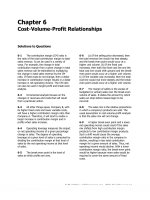
(a) If the selling price decreased, then
the total revenue line would rise less steeply,
and the break-even point would occur at a
higher unit volume. (b) If the fixed cost
increased, then both the fixed cost line and the
total cost line would shift upward and the breakeven point would occur at a higher unit volume.
(c) If the variable cost increased, then the total
cost line would rise more steeply and the breakeven point would occur at a higher unit volume.
6-7
The margin of safety is the excess of
budgeted (or actual) sales over the break-even
volume of sales. It states the amount by which
sales can drop before losses begin to be
incurred.
6-8
The sales mix is the relative proportions
in which a company’s products are sold. The
usual assumption in cost-volume-profit analysis
is that the sales mix will not change.

6-9
A higher break-even point and a lower
net operating income could result if the sales
mix shifted from high contribution margin
products to low contribution margin products.
Such a shift would cause the average
contribution margin ratio in the company to
decline, resulting in less total contribution
margin for a given amount of sales. Thus, net
operating income would decline. With a lower
contribution margin ratio, the break-even point
would be higher because more sales would be
required to cover the same amount of fixed
costs.

© The McGraw-Hill Companies, Inc., 2010. All rights reserved.
Solutions Manual, Chapter 6

257


To download more slides, ebook, solutions and test bank, visit

Brief Exercise 6-1 (20 minutes)
1. The new income statement would be:
Sales (10,100 units) ........
Variable expenses ...........
Contribution margin.........
Fixed expenses ...............
Net operating income ......

Total

Per Unit

$353,500
202,000
151,500
135,000
$ 16,500

$35.00
20.00
$15.00

You can get the same net operating income using the following
approach:
Original net operating income ....
Change in contribution margin
(100 units × $15.00 per unit) ..
New net operating income .........

$15,000
1,500
$16,500

2. The new income statement would be:
Sales (9,900 units) ............
Variable expenses .............
Contribution margin...........

Fixed expenses .................
Net operating income ........

Total

$346,500
198,000
148,500
135,000
$ 13,500

Per Unit

$35.00
20.00
$15.00

You can get the same net operating income using the following
approach:
Original net operating income .............
Change in contribution margin
(-100 units × $15.00 per unit) ..........
New net operating income ..................

$15,000
(1,500)
$13,500

© The McGraw-Hill Companies, Inc., 2010. All rights reserved.
258

Introduction to Managerial Accounting, 5th Edition


To download more slides, ebook, solutions and test bank, visit

Brief Exercise 6-1 (continued)
3. The new income statement would be:
Sales (9,000 units) .......
Variable expenses ........
Contribution margin......
Fixed expenses ............
Net operating income ...

Total Per Unit

$315,000
180,000
135,000
135,000
$
0

$35.00
20.00
$15.00

Note: This is the company’s break-even point.

© The McGraw-Hill Companies, Inc., 2010. All rights reserved.

Solutions Manual, Chapter 6

259


To download more slides, ebook, solutions and test bank, visit

Brief Exercise 6-2 (30 minutes)
1. The CVP graph can be plotted using the three steps outlined in the text.
The graph appears on the next page.
Step 1. Draw a line parallel to the volume axis to represent the total
fixed expense. For this company, the total fixed expense is $24,000.
Step 2. Choose some volume of sales and plot the point representing
total expenses (fixed and variable) at the activity level you have
selected. We’ll use the sales level of 8,000 units.
Fixed expenses ...................................................
Variable expenses (8,000 units × $18 per unit) .....
Total expense .....................................................

$ 24,000
144,000
$168,000

Step 3. Choose some volume of sales and plot the point representing
total sales dollars at the activity level you have selected. We’ll use the
sales level of 8,000 units again.
Total sales revenue (8,000 units × $24 per unit)...

$192,000

2. The break-even point is the point where the total sales revenue and the
total expense lines intersect. This occurs at sales of 4,000 units. This
can be verified as follows:
Profit =
=
=
=

Unit CM × Q − Fixed expenses
($24 − $18) × 4,000 − $24,000
$6 × 4,000 − $24,000
$24,000− $24,000 = $0

© The McGraw-Hill Companies, Inc., 2010. All rights reserved.
260

Introduction to Managerial Accounting, 5th Edition


To download more slides, ebook, solutions and test bank, visit

Brief Exercise 6-2 (continued)

CVP Graph
$200,000

Dollars

$150,000

$100,000

$50,000

$0
0

2,000

4,000

6,000

8,000

Volume in Units
Fixed Expense
Total Sales Revenue

Total Expense

© The McGraw-Hill Companies, Inc., 2010. All rights reserved.
Solutions Manual, Chapter 6

261


To download more slides, ebook, solutions and test bank, visit

Brief Exercise 6-3 (15 minutes)

1. The profit graph is based on the following simple equation:
Profit = Unit CM × Q − Fixed expenses
Profit = ($16 − $11) × Q − $16,000
Profit = $5 × Q − $16,000
To plot the graph, select two different levels of sales such as Q=0 and
Q=4,000. The profit at these two levels of sales are -$16,000 (=$5 × 0
− $16,000) and $4,000 (= $5 × 4,000 − $16,000).

Profit Graph
$5,000

$0

Profit

-$5,000

-$10,000

-$15,000

-$20,000
0

500

1,000 1,500 2,000 2,500 3,000 3,500 4,000
Sales Volume in Units

© The McGraw-Hill Companies, Inc., 2010. All rights reserved.

262

Introduction to Managerial Accounting, 5th Edition


To download more slides, ebook, solutions and test bank, visit

Brief Exercise 6-3 (continued)
2. Looking at the graph, the break-even point appears to be 3,200 units.
This can be verified as follows:
Profit =
=
=
=

Unit CM × Q − Fixed expenses
$5 × Q − $16,000
$5 × 3,200 − $16,000
$16,000 − $16,000 = $0

© The McGraw-Hill Companies, Inc., 2010. All rights reserved.
Solutions Manual, Chapter 6

263


To download more slides, ebook, solutions and test bank, visit

Brief Exercise 6-4 (10 minutes)
1. The company’s contribution margin (CM) ratio is:

Total sales ............................
Total variable expenses .........
= Total contribution margin ...
÷ Total sales .........................
= CM ratio ............................

$200,000
120,000
80,000
$200,000
40%

2. The change in net operating income from an increase in total sales of
$1,000 can be estimated by using the CM ratio as follows:
Change in total sales .......................................
× CM ratio ......................................................
= Estimated change in net operating income ....

$1,000
40 %
$ 400

This computation can be verified as follows:
Total sales ......................
÷ Total units sold ............
= Selling price per unit ....
Increase in total sales ......
÷ Selling price per unit ....
= Increase in unit sales ...
Original total unit sales ....

New total unit sales .........
Total unit sales................
Sales ..............................
Variable expenses ...........
Contribution margin.........
Fixed expenses ...............
Net operating income ......

$200,000
50,000 units
$4.00 per unit
$1,000
$4.00
250
50,000
50,250

per unit
units
units
units

Original

New

50,000
50,250
$200,000 $201,000
120,000 120,600

80,000
80,400
65,000
65,000
$ 15,000 $ 15,400

© The McGraw-Hill Companies, Inc., 2010. All rights reserved.
264

Introduction to Managerial Accounting, 5th Edition


To download more slides, ebook, solutions and test bank, visit

Brief Exercise 6-5 (20 minutes)
1. The following table shows the effect of the proposed change in monthly
advertising budget:

Sales With
Additional
Current Advertising
Sales
Budget
Difference

Sales .............................. $180,000 $189,000
Variable expenses ........... 126,000
132,300
Contribution margin.........
54,000

56,700
Fixed expenses ...............
30,000
35,000
Net operating income ...... $ 24,000 $ 21,700

$ 9,000
6,300
2,700
5,000
($ 2,300)

Assuming no other important factors need to be considered, the
increase in the advertising budget should not be approved because it
would lead to a decrease in net operating income of $2,300.
Alternative Solution 1
Expected total contribution margin:
$189,000 × 30% CM ratio ..................
Present total contribution margin:
$180,000 × 30% CM ratio ..................
Incremental contribution margin ...........
Change in fixed expenses:
Less incremental advertising expense .
Change in net operating income ............

$56,700
54,000
2,700
5,000
($ 2,300)

Alternative Solution 2
Incremental contribution margin:
$9,000 × 30% CM ratio .....................
Less incremental advertising expense ....
Change in net operating income ............

$2,700
5,000
($2,300)

© The McGraw-Hill Companies, Inc., 2010. All rights reserved.
Solutions Manual, Chapter 6

265


To download more slides, ebook, solutions and test bank, visit

Brief Exercise 6-5 (continued)
2. The $2 increase in variable cost will cause the unit contribution margin
to decrease from $27 to $25 with the following impact on net operating
income:
Expected total contribution margin with the
higher-quality components:
2,200 units × $25 per unit .....................
Present total contribution margin:
2,000 units × $27 per unit .....................
Change in total contribution margin ...........

$55,000
54,000
$ 1,000

Assuming no change in fixed costs and all other factors remain the
same, the higher-quality components should be used.

© The McGraw-Hill Companies, Inc., 2010. All rights reserved.
266

Introduction to Managerial Accounting, 5th Edition


To download more slides, ebook, solutions and test bank, visit

Brief Exercise 6-6 (10 minutes)
1. The equation method yields the required unit sales, Q, as follows:
Profit
$10,000
$10,000
$40 × Q
Q
Q

=
=
=
=
=
=

Unit CM × Q − Fixed expenses
($120 − $80) × Q − $50,000
($40) × Q − $50,000
$10,000 + $50,000
$60,000 ÷ $40
1,500 units

2. The formula approach yields the required unit sales as follows:
Units sold to attain = Target profit + Fixed expenses
the target profit
Unit contribution margin
=

$15,000 + $50,000
$40

=

$65,000
= 1,625 units
$40

© The McGraw-Hill Companies, Inc., 2010. All rights reserved.
Solutions Manual, Chapter 6

267


To download more slides, ebook, solutions and test bank, visit

Brief Exercise 6-7 (20 minutes)
1. The equation method yields the break-even point in unit sales, Q, as
follows:
Profit
$0
$0
$3Q
Q
Q

=
=
=
=
=
=

Unit CM × Q − Fixed expenses
($15 − $12) × Q − $4,200
($3) × Q − $4,200
$4,200
$4,200 ÷ $3
1,400 baskets

2. The equation method can be used to compute the break-even point in
sales dollars as follows:
CM ratio =
=

Unit contribution margin
Unit selling price
$3
= 0.20
$15

Profit =
$0 =
0.20 × Sales =
Sales =
Sales =

CM ratio × Sales − Fixed expenses
0.20 × Sales − $4,200
$4,200
$4,200 ÷ 0.20
$21,000

3. The formula method gives an answer that is identical to the equation
method for the break-even point in unit sales:
Unit sales to break even =
=

Fixed expenses
Unit CM
$4,200
= 1,400 baskets
$3

© The McGraw-Hill Companies, Inc., 2010. All rights reserved.

268

Introduction to Managerial Accounting, 5th Edition


To download more slides, ebook, solutions and test bank, visit

Brief Exercise 6-7 (continued)
4. The formula method also gives an answer that is identical to the
equation method for the break-even point in dollar sales:

Dollar sales to break even =
=

Fixed expenses
CM ratio
$4,200
= $21,000
0.20

© The McGraw-Hill Companies, Inc., 2010. All rights reserved.
Solutions Manual, Chapter 6

269


To download more slides, ebook, solutions and test bank, visit

Brief Exercise 6-8 (10 minutes)
1. To compute the margin of safety, we must first compute the break-even

unit sales.
Profit
$0
$0
$10Q
Q
Q

=
=
=
=
=
=

Unit CM × Q − Fixed expenses
($30 − $20) × Q − $7,500
($10) × Q − $7,500
$7,500
$7,500 ÷ $10
750 units

Sales (at the budgeted volume of 1,000 units) ..
Less break-even sales (at 750 units).................
Margin of safety (in dollars) .............................

$30,000
22,500
$ 7,500

2. The margin of safety as a percentage of sales is as follows:
Margin of safety (in dollars) ..............
÷ Sales ............................................
Margin of safety percentage ..............

$7,500
$30,000
25%

© The McGraw-Hill Companies, Inc., 2010. All rights reserved.
270

Introduction to Managerial Accounting, 5th Edition


To download more slides, ebook, solutions and test bank, visit

Brief Exercise 6-9 (20 minutes)
1. The company’s degree of operating leverage would be computed as
follows:
Contribution margin................
÷ Net operating income ..........
Degree of operating leverage ..

$48,000
$10,000
4.8

2. A 5% increase in sales should result in a 24% increase in net operating
income, computed as follows:

Degree of operating leverage .....................................
× Percent increase in sales ........................................
Estimated percent increase in net operating income ....

4.8
5%
24%

3. The new income statement reflecting the change in sales is:

Sales ...........................
Variable expenses ........
Contribution margin......
Fixed expenses ............
Net operating income ...

Amount

$84,000
33,600
50,400
38,000
$12,400

Percent
of Sales

100%
40%
60%

Net operating income reflecting change in sales ......
Original net operating income ................................
Percent change in net operating income .................

$12,400
$10,000
24%

© The McGraw-Hill Companies, Inc., 2010. All rights reserved.
Solutions Manual, Chapter 6

271


To download more slides, ebook, solutions and test bank, visit

Brief Exercise 6-10 (20 minutes)
1. The overall contribution margin ratio can be computed as follows:
Overall CM ratio =
=

Total contribution margin
Total sales
$30,000
=30%
$100,000

2. The overall break-even point in sales dollars can be computed as
follows:

Overall break-even =
=

Total fixed expenses
Overall CM ratio
$24,000
= $80,000
30%

3. To construct the required income statement, we must first determine
the relative sales mix for the two products:
Original dollar sales ......
Percent of total ............
Sales at break-even ......
Sales ...........................
Variable expenses*.......
Contribution margin......
Fixed expenses ............
Net operating income ...

Claimjumper Makeover
$30,000
30%
$24,000

$70,000
70%
$56,000

Claimjumper Makeover

$24,000
16,000
$ 8,000

$56,000
40,000
$16,000

Total

$100,000
100%
$80,000

Total

$80,000
56,000
24,000
24,000
$
0

*Claimjumper variable expenses: ($24,000/$30,000) × $20,000 = $16,000
Makeover variable expenses: ($56,000/$70,000) × $50,000 = $40,000

© The McGraw-Hill Companies, Inc., 2010. All rights reserved.
272

Introduction to Managerial Accounting, 5th Edition

To download more slides, ebook, solutions and test bank, visit

Exercise 6-11 (20 minutes)
1. Sales (20,000 units × 1.15 = 23,000 units) .....
Variable expenses .........................................
Contribution margin.......................................
Fixed expenses .............................................
Net operating income ....................................

Total

Per Unit

$345,000 $ 15.00
207,000
9.00
138,000 $ 6.00
70,000
$ 68,000

2. Sales (20,000 units × 1.25 = 25,000 units) .....
Variable expenses .........................................
Contribution margin.......................................
Fixed expenses .............................................
Net operating income ....................................

$337,500
225,000

112,500
70,000
$ 42,500

$13.50
9.00
$ 4.50

3. Sales (20,000 units × 0.95 = 19,000 units) .....
Variable expenses .........................................
Contribution margin.......................................
Fixed expenses .............................................
Net operating income ....................................

$313,500
171,000
142,500
90,000
$ 52,500

$16.50
9.00
$ 7.50

4. Sales (20,000 units × 0.90 = 18,000 units) .....
Variable expenses .........................................
Contribution margin.......................................
Fixed expenses .............................................
Net operating income ....................................

$302,400
172,800
129,600
70,000
$ 59,600

$16.80
9.60
$ 7.20

© The McGraw-Hill Companies, Inc., 2010. All rights reserved.
Solutions Manual, Chapter 6

273


To download more slides, ebook, solutions and test bank, visit

Exercise 6-12 (30 minutes)
1.

Profit
$0
$0
$18Q
Q
Q

=
=

=
=
=
=

Unit CM × Q − Fixed expenses
($30 − $12) × Q − $216,000
($18) × Q − $216,000
$216,000
$216,000 ÷ $18
12,000 units, or at $30 per unit, $360,000

Alternative solution:
Fixed expenses
Unit sales =
to break even Unit contribution margin
=

$216,000
= 12,000 units
$18

or at $30 per unit, $360,000
2. The contribution margin is $216,000 because the contribution margin is
equal to the fixed expenses at the break-even point.
3. Units sold to attain Target profit + Fixed expenses
=
target profit
Unit contribution margin
=

$90,000 + $216,000
= 17,000 units
$18

Sales (17,000 units × $30 per unit) .......
Variable expenses
(17,000 units × $12 per unit) .............
Contribution margin..............................
Fixed expenses ....................................
Net operating income ...........................

Total

$510,000
204,000
306,000
216,000
$ 90,000

Unit

$30
12
$18

© The McGraw-Hill Companies, Inc., 2010. All rights reserved.
274

Introduction to Managerial Accounting, 5th Edition

To download more slides, ebook, solutions and test bank, visit

Exercise 6-12 (continued)
4. Margin of safety in dollar terms:
Margin of safety = Total sales - Break-even sales
in dollars
= $450,000 - $360,000 = $90,000

Margin of safety in percentage terms:
Margin of safety = Margin of safety in dollars
percentage
Total sales
=

$90,000
= 20%
$450,000

5. The CM ratio is 60%.
Expected total contribution margin: ($500,000 × 60%) .. $300,000
Present total contribution margin: ($450,000 × 60%) .....
270,000
Increased contribution margin ....................................... $ 30,000
Alternative solution:
$50,000 incremental sales × 60% CM ratio = $30,000
Given that the company’s fixed expenses will not change, monthly net
operating income will also increase by $30,000.

© The McGraw-Hill Companies, Inc., 2010. All rights reserved.
Solutions Manual, Chapter 6

275


To download more slides, ebook, solutions and test bank, visit

Exercise 6-13 (30 minutes)
1. Variable expenses: $40 × (100% – 30%) = $28
2. a. Selling price ..........................
Variable expenses .................
Contribution margin ..............
Profit =
$0 =
$12Q =
Q=
Q=

$40 100%
28 70%
$12 30%

Unit CM × Q − Fixed expenses
$12 × Q − $180,000
$180,000
$180,000 ÷ $12
15,000 units

In sales dollars: 15,000 units × $40 per unit = $600,000

Alternative solution:
Profit
$0
0.30 × Sales
Sales
Sales

=
=
=
=
=

CM ratio × Sales − Fixed expenses
0.30 × Sales − $180,000
$180,000
$180,000 ÷ 0.30
$600,000

In units: $600,000 ÷ $40 per unit = 15,000 units
b.

Profit
$60,000
$12Q
$12Q
Q
Q

=

=
=
=
=
=

Unit CM × Q − Fixed expenses
$12 × Q − $180,000
$60,000 + $180,000
$240,000
$240,000 ÷ $12
20,000 units

In sales dollars: 20,000 units × $40 per unit = $800,000

© The McGraw-Hill Companies, Inc., 2010. All rights reserved.
276

Introduction to Managerial Accounting, 5th Edition


To download more slides, ebook, solutions and test bank, visit

Exercise 6-13 (continued)
Alternative solution:
Profit
$60,000
0.30 × Sales
Sales
Sales

=
=
=
=
=

CM ratio × Sales − Fixed expenses
0.30 × Sales − $180,000
$240,000
$240,000 ÷ 0.30
$800,000

In units: $800,000 ÷ $40 per unit = 20,000 units
c. The company’s new cost/revenue relation will be:
Selling price ..............................
Variable expenses ($28 – $4) .....
Contribution margin ...................
Profit
$0
$16Q
Q
Q

=
=
=
=
=

$40 100%
24 60%
$16 40%

Unit CM × Q − Fixed expenses
($40 − $24) × Q − $180,000
$180,000
$180,000 ÷ $16 per unit
11,250 units

In sales dollars: 11,250 units × $40 per unit = $450,000
Alternative solution:
Profit
$0
0.40 × Sales
Sales
Sales

=
=
=
=
=

CM ratio × Sales − Fixed expenses
0.40 × Sales − $180,000
$180,000
$180,000 ÷ 0.40
$450,000

In units: $450,000 ÷ $40 per unit = 11,250 units

© The McGraw-Hill Companies, Inc., 2010. All rights reserved.
Solutions Manual, Chapter 6

277


To download more slides, ebook, solutions and test bank, visit

Exercise 6-13 (continued)
3. a.
Fixed expenses
Unit sales to =
break even
Unit contribution margin
=

$180,000
= 15,000 units
$12 per unit

In sales dollars: 15,000 units × $40 per unit = $600,000
Alternative solution:
Dollar sales to = Fixed expenses
break even
CM ratio
=

$180,000

= $600,000
0.30

In units: $600,000 ÷ $40 per unit = 15,000 units
b.
Unit sales to attain = Fixed expenses + Target profit
target profit
Unit contribution margin
=

$180,000 + $60,000
= 20,000 units
$12 per unit

In sales dollars: 20,000 units × $40 per unit =$800,000
Alternative solution:

Dollar sales to attain = Fixed expenses + Target profit
target profit
CM ratio
$180,000 + $60,000
= $800,000
0.30
In units: $800,000 ÷ $40 per unit = 20,000 units
=

© The McGraw-Hill Companies, Inc., 2010. All rights reserved.
278

Introduction to Managerial Accounting, 5th Edition

To download more slides, ebook, solutions and test bank, visit

Exercise 6-13 (continued)
c.
Fixed expenses
Break-even point =
in unit sales
Unit contribution margin
=

$180,000
=11,250 units
$16 per unit

In sales dollars: 11,250 units × $40 per unit = $450,000
Alternative solution:
Break-even point = Fixed expenses
in sales dollars
CM ratio
=

$180,000
=$450,000
0.40

In units: $450,000 ÷ $40 per unit =11,250 units

© The McGraw-Hill Companies, Inc., 2010. All rights reserved.

Solutions Manual, Chapter 6

279


To download more slides, ebook, solutions and test bank, visit

Exercise 6-14 (20 minutes)
a.
Number of units sold ..
Sales..........................
Variable expenses .......
Contribution margin ....
Fixed expenses ...........
Net operating income..
Number of units sold ..
Sales..........................
Variable expenses .......
Contribution margin ....
Fixed expenses ...........
Net operating income..
b.
Sales ..........................
Variable expenses .......
Contribution margin ....
Fixed expenses ...........
Net operating income ..

Sales .........................
Variable expenses ......

Contribution margin ....
Fixed expenses...........
Net operating income .

Case #1

15,000 *
$180,000 * $12
120,000 *
8
60,000
$4
50,000 *
$ 10,000

Case #2

4,000
$100,000 *
60,000
40,000
32,000 *
$ 8,000 *

Case #3

Case #4

10,000 *
6,000 *

$200,000 $20
$300,000 *
70,000 *
7
210,000
130,000 $13 *
90,000
118,000
100,000 *
$ 12,000 *
($ 10,000) *

Case #1

$500,000 * 100%
400,000
80%
100,000
20% *
93,000
$ 7,000 *

Case #3

$25
15
$10 *

$50
35

$15

Case #2

$400,000 * 100%
260,000 * 65%
140,000
35%
100,000 *
$ 40,000

Case #4

$250,000
100%
$600,000 * 100%
100,000
40%
420,000 * 70%
150,000
60% * 180,000
30%
130,000 *
185,000
$ 20,000 *
($ 5,000) *

*Given

© The McGraw-Hill Companies, Inc., 2010. All rights reserved.

280

Introduction to Managerial Accounting, 5th Edition


To download more slides, ebook, solutions and test bank, visit

Exercise 6-15 (15 minutes)
1.
Sales (15,000 games) .........
Variable expenses ...............
Contribution margin ............
Fixed expenses ...................
Net operating income .........

Total

$300,000
90,000
210,000
182,000
$ 28,000

Per
Unit

$20
6
$14

The degree of operating leverage is:
Degree of operating = Contribution margin
leverage
Net operating income
=

$210,000
= 7.5
$28,000

2. a. Sales of 18,000 games represent a 20% increase over last year’s
sales. Because the degree of operating leverage is 7.5, net operating
income should increase by 7.5 times as much, or by 150% (7.5 ×
20%).
b. The expected total dollar amount of net operating income for next
year would be:
Last year’s net operating income ......................
Expected increase in net operating income next
year (150% × $28,000) ................................
Total expected net operating income ................

$28,000
42,000
$70,000

© The McGraw-Hill Companies, Inc., 2010. All rights reserved.
Solutions Manual, Chapter 6

281