Solution manual managerial accounting 8e by hansen mowen ch 3

To download more slides, ebook, solutions and test bank, visit

CHAPTER 3
ACTIVITY COST BEHAVIOR
QUESTIONS FOR WRITING AND DISCUSSION
1. Knowledge of cost behavior allows a manager to assess changes in costs that result
from changes in activity. This allows a manager to assess the effects of choices that
change activity. For example, if excess capacity exists, bids that at least cover variable
costs may be totally appropriate. Knowing
what costs are variable and what costs are
fixed can help a manager make better bids.
2. The longer the time period, the more likely
that a cost will be variable. The short run is a
period of time for which at least one cost is
fixed. In the long run, all costs are variable.
3. Resource spending is the cost of acquiring
the capacity to perform an activity, whereas
resource usage is the amount of activity actually used. It is possible to use less of the
activity than what is supplied. Only the cost
of the activity actually used should be assigned to products.
4. Flexible resources are those acquired from
outside sources and do not involve any longterm commitment for any given amount of
resource. Thus, the cost of these resources
increases as the demand for them increases, and they are variable costs (varying in
proportion to the associated activity driver).
5. Committed resources are acquired by the
use of either explicit or implicit contracts to
obtain a given quantity of resources, regardless of whether the quantity of resource
available is fully used or not. For multiperiod
commitments, the cost of these resources
essentially corresponds to committed fixed

costs. Other resources acquired in advance
are short term in nature and essentially correspond to discretionary fixed costs.
6. Committed fixed costs are those incurred for
the acquisition of long-term activity capacity
and are not subject to change in the short
run. Annual resource expenditure is independent of actual usage. For example, the
cost of a factory building is a committed
fixed cost. Discretionary fixed costs are
those incurred for the acquisition of shortterm activity capacity, the levels of which
can be altered quickly. In the short run, re-

41

source expenditure is also independent of
actual activity usage. An engineer’s salary is
an example of such an expenditure.
7. A variable cost increases in direct proportion
to changes in activity usage. A one-unit increase in activity usage produces an increase in cost. A step cost, however, increases only as activity usage changes in
small blocks or chunks. An increase in cost
requires an increase in several units of activity. When a step cost changes over relatively
narrow ranges of activity, it may be more
convenient to treat it as a variable cost.
8. A step cost with narrow steps can be treated
as variable, while one with wide steps is typically treated as fixed.
9. An activity rate is the resource expenditure
for an activity divided by the activity’s practical capacity.
10.

Mixed costs are usually reported in total in
the accounting records. How much of the

cost is fixed and how much is variable is unknown and must be estimated.

11.

A scattergraph allows a visual portrayal of
the relationship between cost and activity. It
reveals to the investigator whether a relationship may exist and, if so, whether a linear function can be used to approximate
the relationship. A scattergraph also can assist in identifying any outliers.

12.

Managers can use their knowledge of cost
relationships to estimate fixed and variable
components. A scattergraph can be used as
an aid in this process. From a scattergraph,
a manager can select two points that best
represent the relationship. These two points
can then be used to derive a linear cost formula. The high-low method tells the manager which two points to select to compute the
linear cost formula. The selection of these
two points is not left to judgment.

13.

Because the scatterplot method is not restricted to the high and low points, it is possible to select two points that better represent
the relationship between activity and costs,


To download more slides, ebook, solutions and test bank, visit

producing a better estimate of fixed and variable costs. A scattergraph also identifies

outliers that could represent a high or low
point that is an aberration. The main advantage of the high-low method is that it removes subjectivity from the choice process.
The same line will be produced by two different people.
14.

Assuming that the scattergraph reveals that
a linear cost function is suitable, then the
method of least squares selects a line that
best fits the data points. The method also
provides a measure of goodness of fit so
that the strength of the relationship between
cost and activity can be assessed.

15.

The best-fitting line is the one that is “closest” to the data points. This is usually measured by the line that has the smallest sum of
squared deviations.

16.

No. The best-fitting line may not explain
much of the total cost variability. There must
be a strong relationship as well.

17.

The coefficient of determination is the percentage of total variability in costs explained

42

by the activity. As such, it is a measure of
the goodness of fit, the strength of the relationship between cost and activity.
18.

The correlation coefficient is the square root
of the coefficient of determination. The correlation coefficient reveals the direction of
the relationship in addition to the strength of
the relationship.

19.

If the variation in cost is not well explained
by activity usage (the coefficient of determination is low) as measured by a single driver, then other explanatory variables may be
needed to build a good cost formula.

20.

If the mixed costs are immaterial, then the
method of decomposition is unimportant.
Furthermore, sometimes managerial judgment may be more useful for assigning
costs than the use of formal statistical methodology.


To download more slides, ebook, solutions and test bank, visit

EXERCISES
3–1
1.

Number of Units

0
50,000
100,000
150,000
200,000
250,000

Total Cost
$120,000
120,000
120,000
120,000
120,000
120,000

2.

Supervision cost is strictly fixed.

Cost per Unit
NA
$2.40
1.20
0 .80
0 .60
0 .48

3–2
1.

Miles Traveled
0
$
2,000 600
4,000 1,200
6,000 1,800
8,000 2,400
10,000 3,000

Total Cost
0 $0.00
0.30*
0.30
0.30
0.30
0.30

*$1,200/4,000 or $3,000/10,000 = $.30
2.

The cost of fuel for the delivery activity is strictly variable.

43

Cost per Mile


To download more slides, ebook, solutions and test bank, visit

3–3

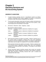
1.

Depreciation Cost

Graph of Truck Depreciation
$250,000
$200,000
$150,000
$100,000
$50,000
$0
0

10 20 30 40 50 60 70 80 90 100

Cubic Yards of Concrete (in
thousands)

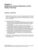
2.

Cost of raw
materials

Graph of Raw Materials Cost
3,000,000
2,000,000

Series2

1,000,000

0
1

2

3 4

5

Cubic yards of concrete

3. Truck depreciation: Fixed cost
Raw materials cost: Variable cost
3-4
1.

Number of Units
0
10,000
20,000
30,000
40,000
50,000

Total Cost
$10,000
10,000
10,000
20,000
20,000

30,000

44

Cost per Unit
NA
$1.00
0.50
0.67
0.50
0.60


To download more slides, ebook, solutions and test bank, visit

2.

Forming machines rental cost is a step cost.

3-5
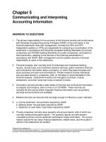
1.
Graph of Machining Direct Labor Cost

Cost of Direct Labor

350000
300000
250000
200000
150000

100000
50000
0
0

1000

2000

3000

4000

5000

Number of units

The direct labor cost in the machining department is a step cost (with narrow
steps).
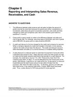
2.

Cost of Supervision

Graph of Machining Department
Supervision Cost
150000
100000
50000
0
0

1000

2000

3000

4000

5000

Number of units

The cost of supervision for the machining department is a step cost (with wide
steps).

45


To download more slides, ebook, solutions and test bank, visit

3. Direct labor cost increase = $144,000 – $108,000 = $36,000
Supervision increase = $80,000 – $40,000 = $40,000

3-6
Cost Category

Variable Cost

Technician

salaries
Laboratory facility
Laboratory
equipment
Chemicals and
other supplies

Discretionary
Fixed Cost
X

Committed Fixed
Cost
X
X

X

3–7
Resource
Jet rental
Hotel rooms
Buffet
Favor package
Buses

Flexible/Committed
Committed
Committed
Flexible

Flexible
Committed

Cost Behavior
Fixed
Fixed
Variable
Variable
Step

3–8
1.

Resource
Plastic1
Direct labor and
variable overhead2
Mold sets3
Other facility costs4
Total

Total Cost
$ 10,800
8,000
20,000
10,000
$48,800

Unit Cost
$0.027

0.020
0.050
0.025
$0.122

1

0.90 × $0.03 × 400,000 = $10,800; $10,800/400,000 = $0.027
$0.02 × 400,000 = $8,000; $8,000/400,000 = $0.02
3
$5,000 × 4 quarters = $20,000; $20,000/400,000 = $0.05
4
$10,000; $10,000/400,000 = $0.025
2

2.

Plastic, direct labor, and variable overhead are flexible resources; molds and
other facility costs are committed resources. The cost of plastic, direct labor,
and variable overhead are strictly variable. The cost of the molds is fixed for
46


To download more slides, ebook, solutions and test bank, visit

the particular action figure being produced; it is a step cost for the production
of action figures in general. Other facility costs are strictly fixed.

3–9
1. Total maintenance cost = $24,000 + $0.30(200,000) = $84,000

2. Total fixed maintenance cost = $24,000
3. Total variable maintenance cost = $0.30(200,000) = $60,000
4. Total maintenance cost per unit = [$24,000 + $0.30(200,000)]/200,000
= $84,000/200,000
= $0.42
5. Fixed maintenance cost per unit = $24,000/200,000 = $0.12
6. Variable maintenance cost per unit = $0.30
7. Requirements1-6 repeated:
1. Total maintenance cost = $24,000 + $0.30(100,000) = $54,000
2. Total fixed maintenance cost = $24,000
3. Total variable maintenance cost = $0.30(100,000) = $30,000
4. Total maintenance cost per unit = [$24,000 + $0.30(100,000)]/100,000
= $54,000/100,000
= $0.54
5. Fixed maintenance cost per unit = $24,000/100,000 = $0.24
6. Variable maintenance cost per unit = $0.30

47


To download more slides, ebook, solutions and test bank, visit

3–10
1.

Committed resources: trucks and technicians’ salaries
Flexible resources: supplies, small tools, and fuel

2.

Variable activity rate = $420,000/35,000 = $12 per call
Fixed activity rate = $600,000*/40,000** = $15 per call
Total cost of one call = $12 + $15 = $27 per call
*($24,000 × 20) + ($10,000 × 12);
**8 × 250 × 20

3.

Activity availability =
Calls available
=
40,000 calls
=

4.

Total cost of
committed resources
$600,000
$600,000

Activity usage
Calls made
35,000 calls

+ Unused capacity
+
Unmade calls
+
5,000 calls

Cost of
= activity used +
= ($15 × 35,000) +
=
$525,000
+

Cost of
unused capacity
($15 × 5,000)
$75,000

Note: The analysis is restricted to committed resources, since only these resources will ever have any unused capacity.

48


To download more slides, ebook, solutions and test bank, visit

3–11
1.

Committed resource charges: monthly fee, activation fee, cancellation fee (if
triggered by contract cancellation prior to one year)
Flexible resource charges: all additional charges for airtime, long distance
and roaming

2.

Plan 1:
Minutes available
60 minutes

=
=

Minutes used
45 minutes

+
+

Unused minutes
15 minutes

Plan 2:
Minutes available
120 minutes

=
=

Minutes used
45 minutes

+
+

Unused minutes

75 minutes

Plan 1 is more cost effective. Jana will have some unused capacity (on average, 15 minutes a month), and the overall cost will be lower by $10 per month.
3.

Plan 1*:
Minutes available
60 minutes

=
=

Minutes used
90 minutes

+
+

Unused minutes
(− 30) minutes

Plan 1*:
Minutes available
=
60 minutes
=
Additional minutes =

Minutes used
60 minutes

30 minutes

+
+

Unused minutes
0 minutes

*There are a number of ways to illustrate the use of minutes with Plan 1. Here
are two possibilities. The problem, of course, is that all included monthly
minutes are used, and Jana must purchase additional minutes.
Plan 2:
Minutes available
120 minutes

=
=

Minutes used
90 minutes

+
+

Unused minutes
30 minutes

Plan 2 is now more cost effective, as the monthly cost is $30. Under Plan 1,
Jana will pay $20 plus $30 (30 minutes × $1.00) or $50 per month. (The $1.00
additional charge includes the airtime and regional roaming charge.)

49


To download more slides, ebook, solutions and test bank, visit

3-12
1.
Graph of Cost of Giving Opening Shows
8000
7000

Cost

6000
5000
4000
3000
2000
1000
0
0

5

10

15

Number of opening shows

This is a strictly variable cost.
2.
Graph of Cost of Running the Gallery
100000

Cost

80000
60000
40000
20000
0
0

5

10

15

20

Number of opening shows

This is a strictly fixed cost.

50

20

To download more slides, ebook, solutions and test bank, visit

3.
Graph of Ben's Total Costs
88000

Total Cost

87000
86000
85000
84000
83000
82000
81000
80000
79000
0

5

10

15

20

Number of opening shows

This is a mixed cost.
4. Total cost = $80,000 + $500(Number of opening shows)
5. Total cost = $80,000 + $500(12) = $86,000
Total cost = $80,000 + $500(14) = $87,000

3-13
1. The high point is March with 3,100 appointments. The low point is January with
700 appointments.
2. Variable rate = ($2,790 – $1,758)/(3,100 – 700)
= $1,032/2,400
= $0.43 per tanning appointment
Using the high point:
Fixed cost = $2,790 – $0.43(3,100) = $1,457
OR

Using the low point:
Fixed cost = $1,758 – $0.43(700) = $1,457
3. Total tanning service cost = $1,457 + $0.43 × Number of appointments
4. Total predicted cost for September = $1,457 + $0.43(2,500) = $2,532

51


To download more slides, ebook, solutions and test bank, visit

Total fixed cost for September = $1,457
Total predicted variable cost = $0.43(2,500) = $1,075

3-14

1.
Scattergraph of Tanning Services
3000

Monthly Cost

2500
2000
1500
1000
500
0
0

1000

2000

3000

4000

Number of appointments

Yes, it appears that there is a linear relationship between tanning cost and number of appointments.
2. Total cost of tanning services = $1,290 + $0.45 × Number of appointments
3. Total predicted cost for September = $1,290 + $0.45(2,500) = $2,415

52

To download more slides, ebook, solutions and test bank, visit

3–15
1.

Cost of Oil Changes
$9,000
$8,000
$7,000

Cost

$6,000
$5,000
$4,000
$3,000
$2,000
$1,000
$0
0

500

1,000

Number of Oil Changes
The scattergraph provides evidence for a linear relationship.
2.

High (1,400, $7,950); Low (700, $5,150)
V = ($7,950 – $5,150)/(1,400 – 700)
= $2,800/700 = $4 per oil change
F = $5,150 – $4(700)
= $5,150 – $2,800 = $2,350
Cost = $2,350 + $4 (oil changes)
Predicted cost for January = $2,350 + $4(1,000) = $6,350

53

1,500


To download more slides, ebook, solutions and test bank, visit

3–15
3.

Concluded

Output of the regression routine calculated by a spreadsheet:
Constant

1697.097

Std. Err. of Y Est.

243.6784

R Squared

0.967026

No. of Observations

8

Degrees of Freedom

6

X Coefficient(s)

4.64678

Std. Err. of Coef.

0.350304

Rounding the coefficients:
Variable rate = $4.65 per oil change
Fixed cost = $1,697
Predicted cost for January = $1,697 + $4.65 (oil changes)
= $1,697 + $4.65(1,000) = $6,347
R2 = 0.97 (rounded)
This says that 97 percent of the variability in the cost of providing oil changes
is explained by the number of oil changes performed.
4.

The least-squares method is better because it uses all eight data points instead of just two.

54


To download more slides, ebook, solutions and test bank, visit

3–16
1.

Cost of Moving Materials
$16,000
$14,000
$12,000
$10,000
$8,000
$6,000
$4,000
$2,000
$0
0

500

1,000

Number of Moves

The scattergraph provides evidence for a linear relationship, but the observation for 300 moves may be an outlier.
2.

High (800, $14,560); Low (100, $3,000)
V = ($14,560 – $3,000)/(800 – 100)
= $11,560/700 = $16.51 per move (rounded)
F = $3,000 – $16.51(100)
= $3,000 – $1,651 = $1,349
Cost = $1,349 + $16.51 (moves)
Predicted cost = $1,349 + $16.51(550) = $10,430 (rounded)

55


To download more slides, ebook, solutions and test bank, visit

3–16
3.

Concluded

Output of the regression routine calculated by a spreadsheet:
Constant

497.50

Std. Err. of Y Est.

987.0073

R Squared

0.926208

No. of Observations

8

Degrees of Freedom

6

X Coefficient(s)

18.425

Std. Err. of Coef.

1.954566

Rounding the coefficients:
Variable rate = $18.43 per move
Fixed cost = $498
Cost = $498 + $18.43 (moves)
= $498 + $18.43(550) = $10,635 (rounded)
R2 = 0.93 (rounded)
This says that 93 percent of the variability in the cost of moving materials is
explained by the number of moves.
4.

Normally, we would prefer the least-squares method since the data appear to
be linear. However, the third observation may be an outlier. If the third obser2
vation (300 moves and $3,400 of cost) is dropped, the R rises to 99 percent.

The new cost formula would be
Cost = $1,411 + $17.28 (moves)
The higher fixed cost is much more in keeping with what we observed with
the scatterplot in requirement 1.

56


To download more slides, ebook, solutions and test bank, visit

3–17
1.

Maintenance cost = $5,750 + $16X

2.

Maintenance cost = $5,750 + $16(650) = $5,750 + $10,400 = $16,150

3.

To obtain the percentage explained, r needs to be squared: 0.89 × 0.89 = 79.21
percent. The relationship appears strong but perhaps could be improved by
searching for another explanatory variable. Leaving about 20 percent of the
variability unexplained may produce less than satisfactory predictions.

4.

Maintenance cost = 12($5,750) + $16(8,400) = $69,000 + $134,400 = $203,400

Note: The fixed cost from the regression results is the fixed cost for the
month (since monthly data were used to estimate the equation). However, the
question asks for the cost for the year. Therefore, the fixed cost from the regression equation must be multiplied by 12.

3–18
1.

Overhead = $2,130 + $17(DLH) + $810(setups) + $26(purchase orders)

2.

Overhead = $2,130 + $17(600) + $810(50) + $26(120)
= $2,130 + $10,200 + $40,500 + $3,120
= $55,950

3.

Since total setup cost is $40,500 for the following month, a 50 percent decrease would reduce setup cost to $20,250, saving $20,250 for the month.

57


To download more slides, ebook, solutions and test bank, visit

3–19
1.

Warranty repair cost = $2,000 + $60(number of defects) - $10(inspection
hours)

2.

Warranty repair cost = $2,000 + $60(100) – $10(150) = $6,500

3.

The number of defects is positively correlated with warranty repair costs. Inspection hours are negatively correlated with warranty repair costs.

4.

In this equation, the independent variables—number of defects and inspection hours—account for 88 percent of the variability in warranty repair costs.
It seems that analysts have identified some very good drivers for warranty repair costs.

58


To download more slides, ebook, solutions and test bank, visit

PROBLEMS
3-20
a. Variable cost
b. Committed fixed cost
c. Discretionary fixed cost
d. Discretionary fixed cost
e. Discretionary fixed cost
f. Variable cost
g. Variable cost
h. Discretionary fixed cost
i. Discretionary fixed cost
j. Committed fixed cost

3-21
1.

Receiving Cost

Scattergraph of Receiving Activity
35000
30000
25000
20000
15000
10000
5000
0
0

500

1000

1500

2000

Number of receiving orders

Yes, the relationship appears to be reasonably linear.
2. Using the high-low method:
Variable receiving cost = ($27,000 – $15,000)/(1,700 – 700) = $12

Fixed receiving cost = $15,000 – $12(700) = $6,600
Predicted cost for 1,475 receiving orders:
Receiving cost = $6,600 + $12(1,475) = $24,300
3. Receiving cost for the quarter = 3($6,600) + $12(4,650)

59


To download more slides, ebook, solutions and test bank, visit

= $19,800 + $55,800
= $75,600
Receiving cost for the year = 12($6,600) + $12(18,000)
= $79,200 + $216,000
= $295,200
4. Receiving cost = $3,212 + $15.15 × Number of receiving orders
Receiving cost = $3,212 + $15.15(1,475) = $25,558
Receiving cost for the quarter = 3($3,212) + $15.15(4,650)
= $9,636 + $70,448
= $80,084
Receiving cost for the year = 12($3,212) + $15.15(18,000)
= $38,544 + $272,700
= $311,244
3-22
1. Results of regressions:

10 Months Data 12 Months Data
Intercept
3,212.121
3,820

Slope
15.15152
15.10
0.8485
0.7451
R2

60


To download more slides, ebook, solutions and test bank, visit

2.

Receiving cost

Scattergraph of Receiving Activity 12 Months Data
35000
30000
25000
20000
15000
10000
5000
0
0

500

1000

1500

2000

Number of receiving orders

The point for the 11th month (1,200 receiving orders and $28,000 total receiving
cost) appears to be an outlier. Since the cost was so much higher in this month
due to an event that is not expected to happen again, this data point could easily
be dropped. Then, data from the 11 remaining months could be used to develop a
cost formula for receiving cost.

61


To download more slides, ebook, solutions and test bank, visit

3. Results for the method of least squares after dropping month 11.
SUMMARY OUTPUT
Regression Statistics
Multiple R
0.926737
R Square
0.858841
Adjusted R
Square
0.843157
2051.781
Standard Error

Observations
11
ANOVA
df
Regression
Residual
Total

1
9
10

SS
2.31E+08
37888233
2.68E+08

Intercept
X Variable 1

Coefficients
3168.56
15.17946

Standard
Error
2565.262
2.051314

MS

2.31E+08
4209804

F
54.7581

t Stat
1.23518
7.399872

P-value
0.248035
4.1E-05

Significance
F

4.1E-05

Lower 95%
-2634.47
10.53906

Upper
95%
8971.589
19.81986

Lower
95.0%

-2634.47
10.53906

Upper
95.0%
8971.589
19.81986

Receiving cost = $3,168.56 + $15.18 × Number of receiving orders
Predicted receiving cost for a month
= $3,168.56 + $15.18(1,475) = $25,559.06
The regression run on the 11 months of data from “typical” months appears to be
better than the one for all 12 months. R2 is higher for the regression without the
outlier (85.88 percent versus 74.512 percent), and the scattergraph gives Joseph
confidence that the data without the outlier describe a relatively linear relationship. Since the storm damage is not expected to recur, month 11 can safely be
dropped from a regression meant to help predict future receiving cost.

62


To download more slides, ebook, solutions and test bank, visit

3–23
1.

Salaries:
Senior accountant—fixed
Office assistant—fixed
Internet and software subscriptions—mixed
Consulting by senior partner—variable

Depreciation (equipment)—fixed
Supplies—mixed
Administration—fixed
Rent (offices)—fixed
Utilities—mixed

2.

Internet and software subscriptions:
V = (Y2 – Y1)/(X2 – X1)
= ($850 – $700)/(150 – 120) = $5 per hour
F = Y2 – VX2
= $850 – ($5)(150) = $100
Consulting by senior partner:
V = (Y2 – Y1)/(X2 – X1)
= ($1,500 – $1,200)/(150 – 120) = $10 per hour
F = Y2 – VX2
= $1,500 – ($10)(150) = $0
Supplies:
V = (Y2 – Y1)/(X2 – X1)
= ($1,100 – $905)/(150 – 120) = $6.50 per hour
F = Y2 – VX2
= $1,100 – ($6.50)(150) = $125
Utilities:
V = (Y2 – Y1)/(X2 – X1)
= ($365 – $332)/(150 – 120) = $1.10 per hour
F = Y2 – VX2
= $365 – ($1.10)(150) = $200

63

To download more slides, ebook, solutions and test bank, visit

3–23

Concluded

3.

Unit
Variable Cost

Fixed
Salaries:
Senior accountant
Office assistant
Internet and subscriptions
Consulting
Depreciation (equipment)
Supplies
Administration
Rent (offices)
Utilities
Total cost

$2,500
1,200
100
—

2,400
125
500
2,000
200
$9,025

$ —
—
5.00
10.00
—
6.50
—
—
1.10
$22.60

Thus, total clinic cost = $9,025 + $22.60/professional hour
For 140 professional hours:
Clinic cost = $9,025 + $22.60(140) = $12,189
Charge per hour = $12,189/140 = $87.06
Fixed charge per hour = $9,025/140 = $64.46
Variable charge per hour = $22.60
4.

For 170 professional hours:
Charge/day = $9,025/170 + $22.60 = $53.09 + $22.60 = $75.69
The charge drops because the fixed costs are spread over more professional
hours.

64


To download more slides, ebook, solutions and test bank, visit

3–24
1.

High (1,700, $21,000); Low (700, $15,000)
V = (Y2 – Y1)/(X2 – X1)
= ($21,000 – $15,000)/(1,700 – 700) = $6 per setup
F = Y2 – VX2
= $21,000 – ($6)(1,700) = $10,800
Y = $10,800 + $6X

2.

Output of spreadsheet regression routine with number of setups as the independent variable:
Constant

4512.98701298698

Std. Err. of Y Est.

3456.24317476605

R Squared

0.633710482694768

No. of Observations

10

Degrees of Freedom

8

X Coefficient(s)

13.3766233766234

Std. Err. of Coef.

3.59557461331427

V = $13.38 per receiving order (rounded)
F = $4,513 (rounded)
Y = $4,513 + $13.38X
R2 = 0.634, or 63.4%
Setups explain about 63.4 percent of the variability in order filling cost, providing evidence that Brett’s choice of a cost driver is reasonable. However,
other drivers may need to be considered because 63.4 percent may not be
strong enough to justify the use of only receiving orders.

65