Solution manual managerial accounting 13e by garrison appa

To download more slides, ebook, solutions and test bank, visit

Appendix A
Pricing Products and Services
Solutions to Questions
A-1
In cost-plus pricing, prices are set by
applying a markup percentage to a product’s
cost.
A-2
The price elasticity of demand measures
the degree to which a change in price affects
unit sales. The unit sales of a product with inelastic demand are relatively insensitive to the
price charged for the product. In contrast, the
unit sales of a product with elastic demand are
sensitive to the price charged for the product.
A-3
The profit-maximizing price should depend only on the variable (marginal) cost per
unit and on the price elasticity of demand. Fixed
costs do not enter into the pricing decision at all.
Fixed costs are relevant in a decision of whether
to offer a product or service at all, but are not
relevant in deciding what to charge for the
product or service once the decision to offer it
has been made. Because price affects unit sales,
total variable costs are affected by the pricing
decision and therefore are relevant.
A-4
The markup over variable cost depends
on the price elasticity of demand. A product
whose demand is elastic should have a lower

markup over cost than a product whose demand
is inelastic. If demand for a product is inelastic,
the price can be increased without cutting as
drastically into unit sales.
A-5
The markup in the absorption costing
approach to pricing is supposed to cover selling
and administrative expenses as well as providing
for an adequate return on the assets tied up in

the product. Full cost is an alternative approach
not discussed in the chapter that is used almost
as frequently as the absorption approach. Under
the full cost approach, all costs—including selling and administrative expenses—are included in
the cost base. If full cost is used, the markup is
only supposed to provide for an adequate return
on the assets.
A-6
The absorption costing approach assumes that consumers do not react to prices at
all—consumers will purchase the forecasted unit
sales regardless of the price that is charged.
This is clearly an unrealistic assumption except
under very special circumstances.
A-7
The protection offered by full cost pricing is an illusion. All costs will be covered only if
actual sales equal or exceed the forecasted sales
on which the absorption costing price is based.
There is no assurance that a sufficient number
of units will be sold.
A-8

Target costing is used to price new
products. The target cost is the expected selling
price of the new product less the desired profit
per unit. The product development team is
charged with the responsibility of ensuring that
actual costs do not exceed this target cost.
This is the reverse of the way most
companies have traditionally approached the
pricing decision. Most companies start with their
full cost and then add their markup to arrive at
the selling price. In contrast to target costing,
this traditional approach ignores how much customers are willing to pay for the product.

.

© The McGraw-Hill Companies, Inc., 2010. All rights reserved.
Solutions Manual, Pricing Appendix

957


To download more slides, ebook, solutions and test bank, visit

Exercise A-1 (30 minutes)
1. Maria makes more money selling the ice cream cones at the lower price,
as shown below:
Unit sales ......................
Sales .............................
Cost of sales @ $0.43 .....
Contribution margin .......

Fixed expenses ..............
Net operating income .....

$1.89 Price

1,500
$2,835.00
645.00
2,190.00
675.00
$1,515.00

$1.49 Price

2,340
$3,486.60
1,006.20
2,480.40
675.00
$1,805.40

2. The price elasticity of demand, as defined in the text, is computed as
follows:
d

=

ln(1+% change in quantity sold)
ln(1+% change in price)

æ2,340-1,500 ÷
ö
ln(1+ çç
)
÷
÷
çè 1,500
ø
=
æ1.49-1.89 ÷
ö
ln(1+ çç
)
÷
çè 1.89 ÷
ø

=

ln(1+0.56000)
ln(1-0.21164)

=

ln(1.56000)
ln(0.78836)

=

0.44469

= -1.87
-0.23780

© The McGraw-Hill Companies, Inc., 2010. All rights reserved.
958

Managerial Accounting, 13th Edition


To download more slides, ebook, solutions and test bank, visit

Exercise A-1 (continued)
3. The profit-maximizing price can be estimated using the following formula from the text:
æε ö
÷
Profit-maximizing price = çç d ÷
Variable cost per unit
÷
çè1+ε ø
÷
d
æ -1.87 ÷
ö
= çç
$0.43
÷
çè1+(-1.87) ÷
ø
= 2.1494 × $0.43 = $0.92

This price is much lower than the prices Maria has been charging in the
past. Rather than immediately dropping the price to $0.92, it would be
prudent to drop the price a bit and see what happens to unit sales and
to profits. The formula assumes that the price elasticity is constant,
which may not be the case.

© The McGraw-Hill Companies, Inc., 2010. All rights reserved.
Solutions Manual, Pricing Appendix

959


To download more slides, ebook, solutions and test bank, visit

Exercise A-2 (15 minutes)
1.
Required ROI + Selling and administraive
(
×
Investment )
expenses
Markup percentage =
on absorption cost

Unit sales × Unit product cost

=
=

(12% × $750,000) + $50,000

14,000 units × $25 per unit
$140,000
= 40%
$350,000

2. Unit product cost ...............
Markup (40% × $25).........
Selling price per unit ..........

$25
10
$35

© The McGraw-Hill Companies, Inc., 2010. All rights reserved.
960

Managerial Accounting, 13th Edition


To download more slides, ebook, solutions and test bank, visit

Exercise A-3 (10 minutes)
Sales (300,000 units × $15 per unit)........
Less desired profit (12% × $5,000,000) ...
Target cost for 300,000 units ...................

$4,500,000
600,000
$3,900,000

Target cost per unit = $3,900,000 ÷ 300,000 units = $13 per unit

© The McGraw-Hill Companies, Inc., 2010. All rights reserved.
Solutions Manual, Pricing Appendix

961


To download more slides, ebook, solutions and test bank, visit

Problem A-4 (45 minutes)
1. a. Supporting computations:
Number of pads manufactured each year:
38,400 labor-hours ÷ 2.4 labor-hours per pad = 16,000 pads.
Selling and administrative expenses:
Variable (16,000 pads × $9 per pad) ....
Fixed ..................................................
Total ...................................................

$144,000
732,000
$876,000

Required ROI + Selling and administrative
(
expenses
Markup percentage = × Investment )
on absorption cost

Unit sales × Unit product cost

=
=

(24% × $1,350,000) + $876,000
16,000 pads × $60 per pad
$1,200,000
= 125%
$960,000

b. Direct materials ......................................
Direct labor ............................................
Manufacturing overhead .........................
Unit product cost ....................................
Add markup: 125% of unit product cost ..
Selling price ...........................................

$ 10.80
19.20
30.00
60.00
75.00
$135.00

© The McGraw-Hill Companies, Inc., 2010. All rights reserved.
962

Managerial Accounting, 13th Edition

To download more slides, ebook, solutions and test bank, visit

Problem A-4 (continued)
c. The income statement will be:
Sales (16,000 pads × $135 per pad) ..............
Cost of goods sold
(16,000 pads × $60 per pad) ......................
Gross margin ................................................
Selling and administrative expenses:
Sales commissions ......................................
Salaries ......................................................
Warehouse rent ..........................................
Advertising and other .................................
Total selling and administrative expense .........
Net operating income ....................................

$2,160,000
960,000
1,200,000
$144,000
82,000
50,000
600,000

876,000
$ 324,000

The company’s ROI computation for the pads will be:
ROI =
=

Net Operating Income
Sales
×
Sales
Average Operating Assets
$324,000
$2,160,000
×
$2,160,000
$1,350,000

= 15% × 1.6 = 24%

2. Variable cost per unit:
Direct materials ..............................................
Direct labor ....................................................
Variable manufacturing overhead (1/5 × $30) ..
Sales commissions ..........................................
Total ..............................................................

$10.80
19.20
6.00
9.00
$45.00

If the company has idle capacity and sales to the retail outlet would not
affect regular sales, any price above the variable cost of $45 per pad
would add to profits. The company should aggressively bargain for more

than this price; $45 is simply the rock-bottom floor below which the
company should not go in its pricing.

© The McGraw-Hill Companies, Inc., 2010. All rights reserved.
Solutions Manual, Pricing Appendix

963


To download more slides, ebook, solutions and test bank, visit

Problem A-5 (45 minutes)
1. The postal service makes more money selling the souvenir sheets at the
lower price, as shown below:
Unit sales ...............................
Sales ......................................
Cost of sales @ $0.80 per unit .
Contribution margin ................

$7 Price

100,000
$700,000
80,000
$620,000

$8 Price

85,000
$680,000

68,000
$612,000

2. The price elasticity of demand, as defined in the text, is computed as
follows:
d

=

ln(1 + % change in quantity sold)
ln(1 + % change in price)

æ85,000 - 100,000 ÷
ö
ln(1 + çç
÷
÷)
çè
100,000
ø
=
æ8 - 7 ö
÷
ln(1 + çç
÷
÷)
çè 7 ø

=

ln(1 - 0.1500)
ln(1 + 0.1429)

=

ln(0.8500)
ln(1.1429)

=

-0.1625
0.1336

= -1.2163

© The McGraw-Hill Companies, Inc., 2010. All rights reserved.
964

Managerial Accounting, 13th Edition


To download more slides, ebook, solutions and test bank, visit

Problem A-5 (continued)
3. The profit-maximizing price can be estimated using the following formula from the text:
æε ö
÷Variable cost per unit
Profit-maximizing price = çç d ÷
çè1+ε ÷
÷

dø

æ -1.2163 ÷
ö
= çç
$0.80
÷
çè1+(-1.2163) ÷
ø

= 5.6232 × $0.80 = $4.50
This price is much lower than the price the postal service has been
charging in the past. Rather than immediately dropping the price to
$4.50, it would be prudent for the postal service to drop the price a bit
and observe what happens to unit sales and to profits. The formula assumes that the price elasticity of demand is constant, which may not be
true.

© The McGraw-Hill Companies, Inc., 2010. All rights reserved.
Solutions Manual, Pricing Appendix

965


To download more slides, ebook, solutions and test bank, visit

Problem A-5 (continued)
The critical assumption in these calculations is that the percentage
increase (decrease) in quantity sold is always the same for a given percentage decrease (increase) in price. If this is true, we can estimate the
demand schedule for souvenir sheets as follows:

Price*

$8.00
$7.00
$6.13
$5.36
$4.69
$4.10
$3.59
$3.14
$2.75
$2.41

Quantity Sold§
85,000
100,000
117,647
138,408
162,833
191,569
225,375
265,147
311,937
366,985

*

The price in each cell in the table is computed by taking 7/8 of the
price just above it in the table. For example, $6.13 is 7/8 of $7.00 and
$5.36 is 7/8 of $6.13.

§
The quantity sold in each cell of the table is computed by multiplying
the quantity sold just above it in the table by 100,000/85,000. For example, 117,647 is computed by multiplying 100,000 by the fraction
100,000/85,000.

© The McGraw-Hill Companies, Inc., 2010. All rights reserved.
966

Managerial Accounting, 13th Edition


To download more slides, ebook, solutions and test bank, visit

Problem A-5 (continued)
The profit at each price in the above demand schedule can be computed as follows:

Price
(a)

$8.00
$7.00
$6.13
$5.36
$4.69
$4.10
$3.59
$3.14
$2.75
$2.41

Quantity
Sold (b)
85,000
100,000
117,647
138,408
162,833
191,569
225,375
265,147
311,937
366,985

Sales
(a) × (b)

$680,000
$700,000
$721,176
$741,867
$763,687
$785,433
$809,096
$832,562
$857,827
$884,434

Cost of Sales
$0.80 × (b)
$68,000

$80,000
$94,118
$110,726
$130,266
$153,255
$180,300
$212,118
$249,550
$293,588

Contribution
Margin
$612,000
$620,000
$627,058
$631,141
$633,421
$632,178
$628,796
$620,444
$608,277
$590,846

© The McGraw-Hill Companies, Inc., 2010. All rights reserved.
Solutions Manual, Pricing Appendix

967


To download more slides, ebook, solutions and test bank, visit

Problem A-5 (continued)
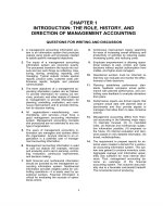
The contribution margin is plotted below as a function of the selling price:

Contribution Margin

$640,000
$630,000
$620,000
$610,000
$600,000
$590,000
$580,000
$2.00

$3.00

$4.00

$5.00

$6.00

$7.00

$8.00

Selling Price

The plot confirms that the profit-maximizing price is about $4.50.

© The McGraw-Hill Companies, Inc., 2010. All rights reserved.
968

Managerial Accounting, 13th Edition


To download more slides, ebook, solutions and test bank, visit

Problem A-5 (continued)
4. If the postal service wants to maximize the contribution margin and
profit from sales of souvenir sheets, the new price should be:
æε ö
÷Variable cost per unit
Profit-maximizing price = çç d ÷
çè1+ε ÷
÷
dø

æ -1.2163 ÷
ö
= çç
$1.00
÷
çè1+(-1.2163) ÷
ø

= 5.6232 × $1.00 = $5.62
Note that a $0.20 increase in cost has led to a $1.12 ($5.62 – $4.50) increase in selling price. This is because the profit-maximizing price is
computed by multiplying the variable cost by 5.6232. Because the variable cost has increased by $0.20, the profit-maximizing price has increased by $0.20 × 5.6232, or $1.12.

Some people may object to such a large increase in price as ―unfair‖
and some may even suggest that only the $0.20 increase in cost should
be passed on to the consumer. The enduring popularity of full-cost pricing may be explained to some degree by the notion that prices should
be ―fair‖ rather than calculated to maximize profits.

© The McGraw-Hill Companies, Inc., 2010. All rights reserved.
Solutions Manual, Pricing Appendix

969


To download more slides, ebook, solutions and test bank, visit

Problem A-6 (60 minutes)
1. The complete, filled-in table appears below:

Selling
Price

$25.00
$23.75
$22.56
$21.43
$20.36
$19.34
$18.37
$17.45
$16.58
$15.75

Estimated
Unit Sales
50,000
54,000
58,320
62,986
68,025
73,467
79,344
85,692
92,547
99,951

Sales

$1,250,000
$1,282,500
$1,315,699
$1,349,790
$1,384,989
$1,420,852
$1,457,549
$1,495,325
$1,534,429
$1,574,228

Variable
Cost

$300,000

$324,000
$349,920
$377,916
$408,150
$440,802
$476,064
$514,152
$555,282
$599,706

Fixed
Expenses

$960,000
$960,000
$960,000
$960,000
$960,000
$960,000
$960,000
$960,000
$960,000
$960,000

Net
Operating
Income
-$10,000
-$1,500
$5,779

$11,874
$16,839
$20,050
$21,485
$21,173
$19,147
$14,522

© The McGraw-Hill Companies, Inc., 2010. All rights reserved.
970

Managerial Accounting, 13th Edition


To download more slides, ebook, solutions and test bank, visit

Problem A-6 (continued)
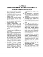
2. A chart based on the above table would look like the following:
$25,000

Net operating income

$20,000
$15,000

$10,000
$5,000
$0
$15
-$5,000

$17

$19

$21

$23

$25

-$10,000
-$15,000
Selling price

Based on this chart, a selling price of about $18 would maximize net operating income.

© The McGraw-Hill Companies, Inc., 2010. All rights reserved.
Solutions Manual, Pricing Appendix

971


To download more slides, ebook, solutions and test bank, visit

Problem A-6 (continued)
3. The price elasticity of demand, as defined in the text, is computed as
follows:
d

=

ln(1 + % change in quantity sold)
ln(1 + % change in price)

=

ln(1+0.08)
ln(1-0.05)

=

ln(1.08)
ln(0.95)

=

0.07696
-0.05129

= -1.500
The profit-maximizing price can be estimated using the following formula from the text:
æ ε ö
÷Variable cost per unit
Profit-maximizing price = çç d ÷
÷
çè1+ε d ÷
ø

æ -1.5 ö

÷
= çç
÷
÷$6.00
çè1+(-1.5) ø

= 3.00 × $6.00 = $18.00
Note that this answer is consistent with the plot of the data in part (2)
above. The formula for the profit-maximizing price works in this case
because the demand is characterized by constant price elasticity. Every
5% decrease in price results in an 8% increase in unit sales.

© The McGraw-Hill Companies, Inc., 2010. All rights reserved.
972

Managerial Accounting, 13th Edition


To download more slides, ebook, solutions and test bank, visit

Problem A-6 (continued)
4. We must first compute the markup percentage, which is a function of
the required ROI of 2%, the investment of $2,000,000, the unit product
cost of $6, and the SG&A expenses of $960,000.
Required ROI + Selling and administrative
expenses
Markup percentage = × Investment
on absorption cost
Unit sales × Unit product cost

(

=

)

(2% × $2,000,000) + $960,000
50,000 units × $6 per unit

= 3.33 (rounded) or 333%

Unit product cost .............
Markup ($6.00 × 3.33) .....
Selling price .....................

$ 6.00
19.98
$25.98

Charging $25.98 (or $26 without rounding) for the software would be a
big mistake if the marketing manager is correct about the effect of price
changes on unit sales. The chart prepared in part (2) above strongly
suggests that the company would lose lots of money selling the software at this price.
Note: It can be shown that the unit sales at the $25.98 price would be
about 47,198 units if the marketing manager is correct about demand.
If so, the company would lose about $16,984 per month:
Sales (47,198 units × $25.98 per unit) .......
Variable cost (47,198 units × $6 per unit) ..
Contribution margin ..................................
Fixed expenses .........................................

Net operating income (loss) .......................

$1,226,204
283,188
943,016
960,000
$ (16,984)

5. If the marketing manager is correct about demand, increasing the price
above $18 per unit will result in a decrease in net operating income and
hence in the return on investment. To increase the net operating income, the owners should look elsewhere. They should attempt to decrease costs or increase the perceived value of the product to more customers so that more units can be sold at any given price or the price
can be increased without sacrificing unit sales.
© The McGraw-Hill Companies, Inc., 2010. All rights reserved.
Solutions Manual, Pricing Appendix

973


To download more slides, ebook, solutions and test bank, visit

Problem A-7 (60 minutes)
1. Supporting computations:
Number of hours worked per year:
20 workers × 40 hours per week × 50 weeks = 40,000 hours
Number of surfboards produced per year:
40,000 hours ÷ 2 hours per surfboard = 20,000 surfboards.
Standard cost per surfboard: $1,600,000 ÷ 20,000 surfboards = $80 per
surfboard.
Fixed manufacturing overhead cost per surfboard:
$600,000 ÷ 20,000 surfboards = $30 per surfboard.

Manufacturing overhead per surfboard: $5 variable + $30 fixed = $35.
Direct labor cost per surfboard: $80 – ($27 + $35) = $18.
Given the computations above, the completed standard cost card would
be as follows:

Direct materials .................
Direct labor .......................
Manufacturing overhead ....
Total standard cost per
surfboard .......................

Standard
Quantity
or Hours
6 feet
2 hours
2 hours

Standard Price
or Rate

$4.50 per foot
$9.00 per hour*
$17.50 per hour**

Standard
Cost
$27
18
35

$80

* $18 ÷ 2 hours = $9 per hour
** $35 ÷ 2 hours = $17.50 per hour

© The McGraw-Hill Companies, Inc., 2010. All rights reserved.
974

Managerial Accounting, 13th Edition


To download more slides, ebook, solutions and test bank, visit

Problem A-7 (continued)
2. a.
Required ROI + Selling and administrative
(
expenses
Markup percentage = × Investment )
on absorption cost

Unit sales × Unit product cost

=
=

(18% × $1,500,000) + $1,130,000
20,000 units × $80 per unit
$1,400,000
= 87.5%

$1,600,000

b. Direct materials ...................
Direct labor .........................
Manufacturing overhead ......
Total cost to manufacture ....
Add markup: 87.5% ............
Selling price ........................

$ 27
18
35
80
70
$150

c. Sales (20,000 boards × $150 per board) ............
Cost of goods sold
(20,000 boards × $80 per board) ....................
Gross margin ....................................................
Selling and administrative expenses ...................
Net operating income ........................................
ROI =
=

$3,000,000
1,600,000
1,400,000
1,130,000
$ 270,000

Net Operating Income
Sales
×
Sales
Average Operating Assets
$270,000
$3,000,000
×
$3,000,000
$1,500,000

= 9% × 2 = 18%

© The McGraw-Hill Companies, Inc., 2010. All rights reserved.
Solutions Manual, Pricing Appendix

975


To download more slides, ebook, solutions and test bank, visit

Problem A-7 (continued)
3. Supporting computations:
Total fixed costs:
Manufacturing overhead ......................................... $ 600,000
Selling and administrative
[$1,130,000 – (20,000 boards × $10 per board)] ..
930,000
Total fixed costs..................................................... $1,530,000

Variable costs per board:
Direct materials .................................
Direct labor .......................................
Variable manufacturing overhead ........
Variable selling ..................................
Variable cost per board ......................

$27
18
5
10
$60

To achieve the 18% ROI, the company would have to sell at least the
20,000 units assumed in part (2) above. The break-even volume can be
computed as follows:
Fixed expenses
Break-even point =
in units sold
Unit contribution margin
=

$1,530,000
$150 per board - $60 per board

= 17,000 boards

© The McGraw-Hill Companies, Inc., 2010. All rights reserved.
976

Managerial Accounting, 13th Edition


To download more slides, ebook, solutions and test bank, visit

Problem A-8 (45 minutes)
1. Projected sales (100 machines × $4,950 per machine) ..
Less desired profit (15% × $600,000) ..........................
Target cost for 100 machines .......................................

$495,000
90,000
$405,000

Target cost per machine ($405,000 ÷ 100 machines) ....
Less National Restaurant Supply’s variable selling cost
per machine .............................................................
Maximum allowable purchase price per machine ...........

$4,050
650
$3,400

2. The relation between the purchase price of the machine and ROI can be
developed as follows:
ROI =
=

Total projected sales - Total cost
Investment

$495,000 - ($650 + Purchase price of machines) × 100
$600,000

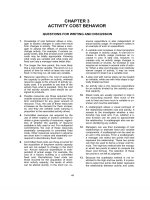
The above formula can be used to compute the ROI for purchase prices
between $3,000 and $4,000 (in increments of $100) as follows:

Purchase price
$3,000
$3,100
$3,200
$3,300
$3,400
$3,500
$3,600
$3,700
$3,800
$3,900
$4,000

ROI

21.7%
20.0%
18.3%
16.7%
15.0%
13.3%
11.7%
10.0%
8.3%

6.7%
5.0%

© The McGraw-Hill Companies, Inc., 2010. All rights reserved.
Solutions Manual, Pricing Appendix

977


To download more slides, ebook, solutions and test bank, visit

Problem A-8 (continued)
Using the above data, the relation between purchase price and ROI can
be plotted as follows:

© The McGraw-Hill Companies, Inc., 2010. All rights reserved.
978

Managerial Accounting, 13th Edition


To download more slides, ebook, solutions and test bank, visit

Problem A-8 (continued)
3. A number of options are available in addition to simply giving up on
adding the new sorbet machines to the company’s product lines. These
options include:
• Check the projected unit sales figures. Perhaps more units could be
sold at the $4,950 price. However, management should be careful not
to indulge in wishful thinking just to make the numbers come out right.

• Modify the selling price. This does not necessarily mean increasing the
projected selling price. Decreasing the selling price may generate
enough additional unit sales to make carrying the sorbet machines
more profitable.
• Improve the selling process to decrease the variable selling costs.
• Rethink the investment that would be required to carry this new product. Can the size of the inventory be reduced? Are the new warehouse
fixtures really necessary?
• Does the company really need a 15% ROI? Does it cost the company
this much to acquire more funds?

© The McGraw-Hill Companies, Inc., 2010. All rights reserved.
Solutions Manual, Pricing Appendix

979