Solutions manual intermediate accounting 18e by stice and stice TVM SOL final

To download more slides, ebook, solutions and test bank, visit

TIME VALUE OF MONEY REVIEW MODULE
EXERCISES
M–1.

M–2.

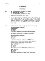
$67,200 [$60,000 + ($60,000 × 0.12 × 1 year)]
$7,200 ($67,200 – $60,000)
$70,800 [$60,000 + ($60,000 × 0.12 × 18/12)]

1.

a.
b.
c.

2.

$71,232 [$67,200 + ($67,200 × 0.12 × 6/12)]

3.

In (1c) simple interest is computed, whereas in (2) interest is compounded annually. The answer in (2) is greater because Dietrick Corporation is paying interest on the interest accumulated in Year 1. The
difference between (1) and (2) of $432 can be computed as being the
interest for 6 months on the $7,200 interest for the first year ($7,200 ×
0.12 × 6/12).

1.

$17,805 ($10,050 × 1.7716, Table I), or ($10,050 ÷ 0.5645, Table II)
Business Calculator Keystrokes:
10050—Press PV
6—Press N
10—Press I
Press FV for the answer = $17,804.1881 = $17,804 (rounded)
Excel Spreadsheet Function:
Using the FV spreadsheet function:
Excel Label
Rate
Nper
Pmt
Pv
Type

Your Input
0.10
6
0
10050
0

Press “Enter” to see the answer of $17,804.
2.

$2,120 ($650 × 3.2620, Table 1), or ($650 ÷ 0.3066, Table II)
Business Calculator Keystrokes:
650—Press PV
40—Press N
3—Press I

Press FV for the answer = $2,120.3246 = $2,120 (rounded)

TVM-1


To download more slides, ebook, solutions and test bank, visit
TVM-2

M–2.

Time Value of Money Module

(Continued)
Excel Spreadsheet Function:
Using the FV spreadsheet function:
Excel Label
Rate
Nper
Pmt
Pv
Type

Your Input
0.03
40
0
650
0

Press “Enter” to see the answer of $2,120.

3.

$16,756 ($5,000 × 1.8106 = $9,053; $9,053 × 1.8509, Table I), or
($5,000 ÷ 0.5523 = $9,053; $9,053 ÷ 0.5403, Table II)
Business Calculator Keystrokes:
5000—Press PV
4—Press N
16—Press I
Press FV for the answer = $9,053.1968 = $9,053 (rounded)
9053—Press PV
8—Press N
8—Press I
Press FV for the answer = $16,756.4712 = $16,756 (rounded)
Excel Spreadsheet Function:
Using the FV spreadsheet function:
Excel Label
Rate
Nper
Pmt
Pv
Type

Your Input
0.16
4
0
5000
0

Press “Enter” to see the answer of $9,053.

Using the FV spreadsheet function:
Excel Label
Rate
Nper
Pmt
Pv
Type

Your Input
0.08
8
0
9053
0

Press “Enter” to see the answer of $16,756.


To download more slides, ebook, solutions and test bank, visit
Time Value of Money Module

M–2.

TVM-3

(Concluded)
4.

$3,536 ($1,000 × 1.4802 = $1,480; $1,480 + $1,000 = $2,480; $2,480 ×
1.4258, Table 1), or ($1,000 ÷ 0.6756 = $1,480; $1,480 + $1,000 = $2,480;

$2,480 ÷ 0.7014, Table II)
Business Calculator Keystrokes:
1000—Press PV
10—Press N
4—Press I
Press FV for the answer = $1,480.2443 = $1,480 (rounded)
2480—Press PV ($1,480 + $1,000 additional investment)
12—Press N
3—Press I
Press FV for the answer = $3,535.8870 = $3,536 (rounded)
Excel Spreadsheet Function:
Using the FV spreadsheet function:
Excel Label
Rate
Nper
Pmt
Pv
Type

Your Input
0.04
10
0
1000
0

Press “Enter” to see the answer of $1,480.
Using the FV spreadsheet function:
Excel Label
Rate

Nper
Pmt
Pv
Type

Your Input
0.03
12
0
2480
0

Press “Enter” to see the answer of $3,536.
M–3.

1.

$9,413 ($17,000 ÷ 1.8061, Table I), or ($17,000 × 0.5537, Table II)
Business Calculator Keystrokes:
17000—Press FV
20—Press N
3—Press I
Press PV for the answer = $9,412.4878 = $9,412 (rounded)


To download more slides, ebook, solutions and test bank, visit
TVM-4

M–3.

Time Value of Money Module

(Continued)
Excel Spreadsheet Function:
Using the PV spreadsheet function:
Excel Label
Rate
Nper
Pmt
Fv
Type

Your Input
0.03
20
0
17000
0

Press “Enter” to see the answer of $9,412.
2.

$4,102 ($5,000 ÷ 1.2190, Table I), or ($5,000 × 0.8203, Table II)
Business Calculator Keystrokes:
5000—Press FV
10—Press N
2—Press I
Press PV for the answer = $4,101.7415 = $4,102 (rounded)
Excel Spreadsheet Function:
Using the PV spreadsheet function:

Excel Label
Rate
Nper
Pmt
Fv
Type

Your Input
0.02
10
0
5000
0

Press “Enter” to see the answer of $4,102.
3.

$1,987 ($25,000 ÷ 2.1911 = $11,410; $11,410 ÷ 5.7435, Table I), or
($25,000 × 0.4564 = $11,410; $11,410 × 0.1741, Table II)
Business Calculator Keystrokes:
25000—Press FV
20—Press N
4—Press I
Press PV for the answer = $11,409.6737 = $11,410 (rounded)
11410—Press FV
30—Press N
6—Press I
Press PV for the answer = $1,986.5966 = $1,987 (rounded)

To download more slides, ebook, solutions and test bank, visit
Time Value of Money Module

M–3.

TVM-5

(Continued)
Excel Spreadsheet Function:
Using the PV spreadsheet function:
Excel Label
Rate
Nper
Pmt
Fv
Type

Your Input
0.04
20
0
25000
0

Press “Enter” to see the answer of $11,410.
Using the PV spreadsheet function:
Excel Label
Rate
Nper
Pmt

Fv
Type

Your Input
0.06
30
0
11410
0

Press “Enter” to see the answer of $1,987.
4.

$3,856 ($12,500 ÷ 1.2653 = $9,879, Table I), or ($12,500 × 0.7903 =
$9,879, Table II) ($9,879 – $5,000 = $4,879; $4,879 ÷ 1.2653, Table 1), or
($4,879 × 0.7903, Table II)
Business Calculator Keystrokes:
12500—Press FV
6—Press N
4—Press I
Press PV for the answer = $9,878.9316 = $9,879 (rounded)
4879—Press FV ($9,879 – $5,000 additional investment)
6—Press N
4—Press I
Press PV for the answer = $3,855.9446 = $3,856 (rounded)


To download more slides, ebook, solutions and test bank, visit
TVM-6

M–3.

Time Value of Money Module

(Concluded)
Excel Spreadsheet Function:
Using the PV spreadsheet function:
Excel Label
Rate
Nper
Pmt
Fv
Type

Your Input
0.04
6
0
12500
0

Press “Enter” to see the answer of $9,879.
Using the PV spreadsheet function:
Excel Label
Rate
Nper
Pmt
Fv
Type

Your Input
0.04
6
0
4879
0

Press “Enter” to see the answer of $3,856.
M–4.

1st Alternative = $14,641 ($10,000 × 1.4641, Table 1), or
($10,000 ÷ 0.6830, Table II)
Business Calculator Keystrokes:
10000—Press PV
4—Press N
10—Press I
Press FV for the answer = $14,641.0000 = $14,641 (rounded)
Excel Spreadsheet Function:
Using the FV spreadsheet function:
Excel Label
Rate
Nper
Pmt
Pv
Type

Your Input
0.10
4
0

10000
0

Press “Enter” to see the answer of $14,641.


To download more slides, ebook, solutions and test bank, visit
Time Value of Money Module

M–4.

TVM-7

(Concluded)
2nd Alternative = $13,728 ($10,000 × 1.3728, Table I), or
($10,000 ÷ 0.7284, Table II)
Business Calculator Keystrokes:
10000—Press PV
16—Press N
2—Press I
Press FV for the answer = $13,727.8571 = $13,728 (rounded)
Excel Spreadsheet Function:
Using the FV spreadsheet function:
Excel Label
Rate
Nper
Pmt
Pv
Type

Your Input
0.02
16
0
10000
0

Press “Enter” to see the answer of $13,728.
M–5.

$2,499 ($30,000 ÷ 12.0061, Table III)
Business Calculator Keystrokes:
30000—Press FV
10—Press N
4—Press I
Press PMT for the answer = $2,498.72833 = $2,499 (rounded)
Excel Spreadsheet Function:
Using the PMT spreadsheet function:
Excel Label
Rate
Nper
Pv

Fv
Type

Your Input
0.04
10
0—this amount would represent

a separate, initial payment in
addition to the regular payments
30000
0

Press “Enter” to see the answer of $2,499.


To download more slides, ebook, solutions and test bank, visit
TVM-8

M–6.

Time Value of Money Module

1.

14 periods, 7 years ($10,000 ÷ $5,051 = 1.9798, Table I), or
($5,051 ÷ $10,000 = 0.5051, Table II)
Business Calculator Keystrokes:
–5051—Press PV (enter as a negative number, signifying an initial
cash outflow)
10000—Press FV
5—Press I
Press N for the answer = 13.9987 periods = 14 periods (rounded)
Excel Spreadsheet Function:
Using the NPER spreadsheet function:
Excel Label
Rate
Pmt

Pv
Fv
Type

Your Input
0.05
0
–5051 (input as a negative number to
signify an initial cash outflow)
10000
0

Press “Enter” to see the answer of 14 periods.
2.

9 periods, 9 years

($10,000 ÷ $5,002 = 1.9992, Table I), or
($5,002 ÷ $10,000 = 0.5002, Table II)

Business Calculator Keystrokes:
–5002—Press PV (enter as a negative number, signifying an initial
cash outflow)
10000— Press FV
8—Press I
Press N for the answer = 9.0013 periods = 9 periods (rounded)
Excel Spreadsheet Function:
Using the NPER spreadsheet function:
Excel Label
Rate

Pmt
Pv
Fv
Type

Your Input
0.08
0
–5002 (input as a negative number to
signify an initial cash outflow)
10000
0

Press “Enter” to see the answer of 9 periods.


To download more slides, ebook, solutions and test bank, visit
Time Value of Money Module

M–6.

TVM-9

(Concluded)
3.

17 periods, 4¼ years ($10,000 ÷ $5,134 = 1.9478, Table I), or
($5,134 ÷ $10,000 = 0.5134, Table II)
Business Calculator Keystrokes:
–5134—Press PV (enter as a negative number, signifying an initial

cash outflow)
10000—Press FV
4—Press I
Press N for the answer = 16.9987 periods = 17 periods (rounded)
Excel Spreadsheet Function:
Using the NPER spreadsheet function:
Excel Label
Rate
Pmt
Pv
Fv
Type

Your Input
0.04
0
–5134 (input as a negative number to
signify an initial cash outflow)
10000
0

Press “Enter” to see the answer of 17 periods.
M–7.

1.

8% ($50,000 ÷ $10,414 = 4.8012, Table I), or
($10,414 ÷ $50,000 = 0.2083, Table II)
Business Calculator Keystrokes:
–10414—Press PV (enter as a negative number, signifying an initial

cash outflow)
50000—Press FV
40—Press N
Press I for the answer = 4.0001% = 4% (rounded) × 2 = 8%
Excel Spreadsheet Function:
Using the RATE spreadsheet function:
Excel Label
Nper
Pmt
Pv
Fv
Type

Your Input
40
0
–10414 (input as a negative number to
signify an initial cash outflow)
50000
0

Press “Enter” to see the answer of 4% × 2 = 8%.


To download more slides, ebook, solutions and test bank, visit
TVM-10

M–7.

Time Value of Money Module

(Concluded)
2.

20% ($50,000 ÷ $7,102 = 7.0403, Table I), or
($7,102 ÷ $50,000 = 0.1420, Table II)
Business Calculator Keystrokes:
–7102—Press PV (enter as a negative number, signifying an initial
cash outflow)
50000—Press FV
40—Press N
Press I for the answer = 5.0001% = 5% (rounded) × 4 = 20%
Excel Spreadsheet Function:
Using the RATE spreadsheet function:
Excel Label
Nper
Pmt
Pv
Fv
Type

Your Input
40
0
–7102 (input as a negative number to
signify an initial cash outflow)
50000
0

Press “Enter” to see the answer of 5% × 4 = 20%.

3.

4% ($50,000 ÷ $33,778 = 1.4803, Table I), or
($33,778 ÷ $50,000 = 0.6756, Table II)
Business Calculator Keystrokes:
–33778—Press PV (enter as a negative number, signifying an initial
cash outflow)
50000—Press FV
10—Press N
Press I for the answer = 4.00006% = 4% (rounded)
Excel Spreadsheet Function:
Using the RATE spreadsheet function:
Excel Label
Nper
Pmt
Pv
Fv
Type

Your Input
10
0
–33778 (input as a negative number to
signify an initial cash outflow)
50000
0

Press “Enter” to see the answer of 4%.

To download more slides, ebook, solutions and test bank, visit
Time Value of Money Module

M–8.

1.

TVM-11

3 periods, 3 years ($20,000 ÷ $5,927 = 3.3744, Table III)
Business Calculator Keystrokes:
–5927—Press PMT (enter as a negative number, signifying a continuing cash outflow)
20000—Press FV
12—Press I
Press N for the answer = 2.999991 periods = 3 periods (rounded)
Excel Spreadsheet Function:
Using the NPER spreadsheet function:
Excel Label
Rate
Pmt
Pv
Fv
Type

Your Input
0.12
–5927 (input as a negative number to
signify regular cash outflows)
0
20000

0

Press “Enter” to see the answer of 3 periods.
2.

5 periods, 2½ years ($20,000 ÷ $3,409 = 5.8668, Table III)
Business Calculator Keystrokes:
–3409—Press PMT (enter as a negative number, signifying a continuing cash outflow)
20000—Press FV
8—Press I
Press N for the answer = 5.0002 periods = 5 periods (rounded)
Excel Spreadsheet Function:
Using the NPER spreadsheet function:
Excel Label
Rate
Pmt
Pv
Fv
Type

Your Input
0.08
–3409 (input as a negative number to
signify regular cash outflows)
0
20000
0

Press “Enter” to see the answer of 5 periods.

To download more slides, ebook, solutions and test bank, visit
TVM-12

M–8.

Time Value of Money Module

(Concluded)
3.

4 periods, 1 year ($20,000 ÷ $4,640 = 4.3103, Table III)
Business Calculator Keystrokes:
–4640—Press PMT (enter as a negative number, signifying a continuing cash outflow)
20000—Press FV
5—Press I
Press N for the answer = 4.0002 periods = 4 periods (rounded)
Excel Spreadsheet Function:
Using the NPER spreadsheet function:
Excel Label
Rate
Pmt
Pv
Fv
Type

Your Input
0.05
–4640 (input as a negative number to
signify regular cash outflows)

0
20000
0

Press “Enter” to see the answer of 4 periods.
M–9.

1.

10% annual rate ($25,000 ÷ $4,095 = 6.1050, Table III)
Business Calculator Keystrokes:
–4095—Press PMT (enter as a negative number, signifying a continuing cash outflow)
25000—Press FV
5—Press N
Press I for the answer = 9.9992% = 10% (rounded)
Excel Spreadsheet Function:
Using the RATE spreadsheet function:
Excel Label
Nper
Pmt
Pv
Fv
Type

Your Input
5
–4095 (input as a negative number to
signify regular cash outflows)
0
25000

0

Press “Enter” to see the answer of 10%.


To download more slides, ebook, solutions and test bank, visit
Time Value of Money Module

M–9.

TVM-13

(Concluded)
2.

12% annual rate ($25,000 ÷ $5,715 = 4.3745, Table III)
Business Calculator Keystrokes:
–5715—Press PMT (enter as a negative number, signifying a continuing cash outflow)
25000—Press FV
4—Press N
Press I for the answer = 5.9975% = 6% (rounded) × 2 = 12%
Excel Spreadsheet Function:
Using the RATE spreadsheet function:
Excel Label
Nper
Pmt
Pv
Fv
Type

Your Input
4
–5715 (input as a negative number to
signify regular cash outflows)
0
25000
0

Press “Enter” to see the answer of 6% × 2 = 12%.
3.

8% annual rate ($25,000 ÷ $1,864 = 13.4120, Table III)
Business Calculator Keystrokes:
–1864—Press PMT (enter as a negative number, signifying a continuing cash outflow)
25000—Press FV
12—Press N
Press I for the answer = 1.999904% = 2% (rounded) × 4 = 8%
Excel Spreadsheet Function:
Using the RATE spreadsheet function:
Excel Label
Nper
Pmt
Pv
Fv
Type

Your Input
12
–1864 (input as a negative number to
signify regular cash outflows)

0
25000
0

Press “Enter” to see the answer of 2% × 4 = 8%.


To download more slides, ebook, solutions and test bank, visit
TVM-14

M–10.

Time Value of Money Module

1.

$228 ($2,410 ÷ 10.5753, Table IV)
Business Calculator Keystrokes:
2410—Press PV
12—Press N
2—Press I
Press PMT for the answer = $227.8886 = $228 (rounded)
Excel Spreadsheet Function:
Using the PMT spreadsheet function:
Excel Label
Rate
Nper
Pv
Fv

Type

Your Input
0.02
12
2410
0—this amount would represent a final
balloon payment to be made at the end
of the loan period, in addition to the
regular payments
0

Press “Enter” to see the answer of $228.
2.

$1,957 ($26,565 ÷ 13.5777, Table IV)
Business Calculator Keystrokes:
26565—Press PV
16—Press N
2—Press I
Press PMT for the answer = $1,956.5156 = $1,957 (rounded)
Excel Spreadsheet Function:
Using the PMT spreadsheet function:
Excel Label
Rate
Nper
Pv
Fv

Type

Your Input
0.02
16
26565
0—this amount would represent a final
balloon payment to be made at the end
of the loan period, in addition to the
regular payments
0

Press “Enter” to see the answer of $1,957.


To download more slides, ebook, solutions and test bank, visit
Time Value of Money Module

M–10.

TVM-15

(Concluded)
3.

$5,256 ($65,500 ÷ 12.4622, Table IV)
Business Calculator Keystrokes:
65500—Press PV
20—Press N
5—Press I
Press PMT for the answer = $5,255.8895 = $5,256 (rounded)

Excel Spreadsheet Function:
Using the PMT spreadsheet function:
Excel Label
Rate
Nper
Pv
Fv

Type

Your Input
0.05
20
65500
0—this amount would represent
a final balloon payment to be
made at the end of the loan period, in addition to the regular
payments
0

Press “Enter” to see the answer of $5,256.
M–11.

1.

$14,403 ($3,000 × 4.8010, Table I), or ($3,000 ÷ 0.2083, Table II)
Business Calculator Keystrokes:
3000—Press PV
40—Press N
4—Press I

Press FV for the answer = $14,403.0619 = $14,403 (rounded)
Excel Spreadsheet Function:
Using the FV spreadsheet function:
Excel Label
Rate
Nper
Pmt
Pv
Type

Your Input
0.04
40
0
3000
0

Press “Enter” to see the answer of $14,403.


To download more slides, ebook, solutions and test bank, visit
TVM-16

M–11.

Time Value of Money Module

(Continued)
2.

$10,747 ($1,000,000 ÷ 93.0510, Table I), or
$10,700 ($1,000,000 × 0.0107, Table II)
Business Calculator Keystrokes:
1000000—Press FV
40—Press N
12—Press I
Press PV for the answer = $10,746.7982 = $10,747 (rounded)
Excel Spreadsheet Function:
Using the PV spreadsheet function:
Excel Label
Rate
Nper
Pmt
Fv
Type

Your Input
0.12
40
0
1000000
0

Press “Enter” to see the answer of $10,747.
3.

n = 25 ($100,000 ÷ $16,401.24 = 6.0971, Table IV)
Business Calculator Keystrokes:
–16401.24—Press PMT (enter as a negative number, signifying a continuing cash outflow)
100000—Press PV

16—Press I
Press N for the answer = 25.00035 periods = 25 periods (rounded)
Excel Spreadsheet Function:
Using the NPER spreadsheet function:
Excel Label
Rate
Pmt

Pv
Fv
Type

Your Input
0.16
–16401.24 (input as a negative
number to signify regular cash
outflows)
100000
0
0

Press “Enter” to see the answer of 25 periods.


To download more slides, ebook, solutions and test bank, visit
Time Value of Money Module

M–11.

TVM-17

(Concluded)
4.

8% ($21,589 ÷ $10,000 = 2.1589, Table I), or
($10,000 ÷ $21,589 = 0.4632, Table II)
Business Calculator Keystrokes:
–10000—Press PV (enter as a negative number, signifying an initial
cash outflow)
21589—Press FV
10—Press N
Press I for the answer = 7.999875% = 8% (rounded)
Excel Spreadsheet Function:
Using the RATE spreadsheet function:
Excel Label
Nper
Pmt
Pv

Fv
Type

Your Input
10
0
–10000 (input as a negative
number to signify an initial cash
outflow)
21589
0

Press “Enter” to see the answer of 8%.
M–12.

1.

$4,438 ($20,000 ÷ 4.5061, Table III)
Business Calculator Keystrokes:
20000—Press FV
4—Press N
8—Press I
Press PMT for the answer = $4,438.4161 = $4,438 (rounded)
Excel Spreadsheet Function:
Using the PMT spreadsheet function:
Excel Label
Rate
Nper
Pv
Fv
Type

Your Input
0.08
4
0
20000
0

Press “Enter” to see the answer of $4,438.

To download more slides, ebook, solutions and test bank, visit
TVM-18

M–12.

Time Value of Money Module

(Continued)
2.

35 payments ($15,850 ÷ $585 = 27.0940, Table IV—The annuity factor
for 1.5% lies between the factors for 1 and 2% where n = 35)
Business Calculator Keystrokes:
–585—Press PMT (enter as a negative number, signifying a continuing
cash outflow)
15850—Press PV
1.5—Press I
Press N for the answer = 35.0313 periods = 35 periods (rounded)
Excel Spreadsheet Function:
Using the NPER spreadsheet function:
Excel Label
Rate
Pmt
Pv
Fv
Type

Your Input
0.015

–585 (input as a negative number to
signify regular cash outflows)
15850
0
0

Press “Enter” to see the answer of 35 periods.
3.

Approximately 12% annually, compounded semiannually
($7,726 ÷ $250 = 30.9040, Table III)
Business Calculator Keystrokes:
–250—Press PMT (enter as a negative number, signifying a continuing
cash outflow)
7726—Press FV
18—Press N
Press I for the answer = 5.9994% = 6% (rounded) × 2 = 12%
Excel Spreadsheet Function:
Using the RATE spreadsheet function:
Excel Label
Nper
Pmt
Pv
Fv
Type

Your Input
18
–250 (input as a negative number to
signify regular cash outflows)

0
7726
0

Press “Enter” to see the answer of 6% × 2 = 12%.


To download more slides, ebook, solutions and test bank, visit
Time Value of Money Module

M–12.

TVM-19

(Concluded)
4.

7 periods, 7 years ($50,445 ÷ $5,000 = 10.0890, Table III)
Business Calculator Keystrokes:
–5000—Press PMT (enter as a negative number, signifying a continuing cash outflow)
50445—Press FV
12—Press I
Press N for the answer = 6.999994 periods = 7 periods (rounded)
Excel Spreadsheet Function:
Using the NPER spreadsheet function:
Excel Label
Rate
Pmt
Pv
Fv

Type

Your Input
0.12
–5000 (input as a negative number to
signify regular cash outflows)
0
50445
0

Press “Enter” to see the answer of 7 periods.
M–13.

4% ($2,500 ÷ $2,404 ≈ 1.0400, Table I), or ($2,404 ÷ $2,500 = 0.9616, Table II)
Annual Rate = 4% × 2 = 8%
Business Calculator Keystrokes:
–2404—Press PV (enter as a negative number, signifying an initial cash
outflow)
2500—Press FV
1—Press N
Press I for the answer = 3.9933% = 4% (rounded) × 2 = 8%
Excel Spreadsheet Function:
Using the RATE spreadsheet function:
Excel Label
Nper
Pmt
Pv
Fv
Type

Your Input
1
0
–2404 (input as a negative number to
signify an initial cash outflow)
2500
0

Press “Enter” to see the answer of 4% × 2 = 8%.


To download more slides, ebook, solutions and test bank, visit
TVM-20

M–14.

Time Value of Money Module

Option A = $40,879 ($5,700 × 3.3121 = $18,879, Table IV; $18,879 + $22,000)
Business Calculator Keystrokes:
5700—Press PMT
4—Press N
8—Press I
Press PV for the answer = $18,879.1230 = $18,879 (rounded) + $22,000 =
$40,879
Excel Spreadsheet Function:
Using the PV spreadsheet function:
Excel Label
Rate
Nper

Pmt
Fv
Type

Your Input
0.08
4
5700
0
0

Press “Enter” to see the answer of $18,879 + $22,000 = $40,879.
Option B = $39,809 ($9,000 × 3.3121 = $29,809, Table IV; $29,809 + $10,000)
Business Calculator Keystrokes:
9000—Press PMT
4—Press N
8—Press I
Press PV for the answer = $29,809.1416 = $29,809 (rounded) + $10,000 =
$39,809
Excel Spreadsheet Function:
Using the PV spreadsheet function:
Excel Label
Rate
Nper
Pmt
Fv
Type

Your Input
0.08

4
9000
0
0

Press “Enter” to see the answer of $29,809 + $10,000 = $39,809.
Other things being equal, Foot Loose should purchase from Do-It-Yourself
Machines (Option B).


To download more slides, ebook, solutions and test bank, visit
Time Value of Money Module

M–15.

TVM-21

Plan A = $13,311 ($15,000 × 0.8874, Table II)
Business Calculator Keystrokes:
15000—Press FV
12—Press N
1—Press I
Press PV for the answer = $13,311.7384 = $13,312 (rounded)
Excel Spreadsheet Function:
Using the PV spreadsheet function:
Excel Label
Rate
Nper
Pmt
Fv

Type

Your Input
0.01
12
0
15000
0

Press “Enter” to see the answer of $13,312.
Plan B = $13,506 ($1,200 × 11.2551, Table IV)
Business Calculator Keystrokes:
1200—Press PMT
12—Press N
1—Press I
Press PV for the answer = $13,506.0930 = $13,506 (rounded)
Excel Spreadsheet Function:
Using the PV spreadsheet function:
Excel Label
Rate
Nper
Pmt
Fv
Type

Your Input
0.01
12
1200
0

0

Press “Enter” to see the answer of $13,506.
Other things being equal, Park City should choose Plan B because it would
earn slightly more rent revenue. However, the cost of processing monthly
checks might exceed the extra revenue received.


To download more slides, ebook, solutions and test bank, visit
TVM-22

M–16.

Time Value of Money Module

1.

a.

1 − (1 + 0.01)

–120

= 69.7005;

$300,000
=
69.7005

=

$300,000
= $55,287.31
5.4262

0.01

b.

1 − (1 + 0.13)

–10

5.4262;

0.13

2.

$4,304.13

The effective annual interest rate associated with the mortgage involving monthly payments is 12.68% = 1.0112 (see Table III, column 1%,
row 12), while the rate associated with the mortgage involving annual
payments is 13%. Thus, the Shrubs would be better off to take the 12%
mortgage with monthly payments.
Another way to illustrate the difference is to compute the future value
of the 12 monthly payments and compare that to the annual payment
of $55,287.31. The monthly payment of $4,304.13 × 12.6825 (Table III) =
$54,587.13 is less than the annual payment of $55,287.31.

M–17.

Plan A

= $375

Plan B

= $402.90 ($55 × 7.3255, Table IV)

Business Calculator Keystrokes:
55—Press PMT
8—Press N
2—Press I
Press PV for the answer = $402.9015 = $402.90 (rounded)
Excel Spreadsheet Function:
Using the PV spreadsheet function:
Excel Label
Rate
Nper
Pmt
Fv
Type

Your Input
0.02
8
55
0
0

Press “Enter” to see the answer of $402.90.
Plan C

= $380.07 [$100 + ($50 × 5.6014, Table IV)]

Business Calculator Keystrokes:
50—Press PMT
6—Press N
2—Press I
Press PV for the answer = $280.0715 = $280.07 (rounded) + $100.00 =
$380.07


To download more slides, ebook, solutions and test bank, visit
Time Value of Money Module

M–17.

TVM-23

(Concluded)
Excel Spreadsheet Function:
Using the PV spreadsheet function:
Excel Label
Rate
Nper
Pmt
Fv
Type

Your Input
0.02
6
50
0
0

Press “Enter” to see the answer of $280.07 + $100.00 = $380.07.
If you were the purchaser, you would choose Plan A—pay $375 cash for the
new freezer. If you were the seller, you would want the customer to choose
Plan B—8 monthly payments of $55.
M–18.

$92,517 ($28,000 × 5.5824 = $156,307, Table IV; $156,307 ÷ 1.6895 = $92,517,
Table 1), or ($28,000 × 5.9173 = $165,684, Table VI; $165,684 × 0.5584 =
$92,518, Table II)
Business Calculator Keystrokes:
28000—Press PMT
7—Press N
6—Press I
Press PV for the answer = $156,306.6803 = $156,307 (rounded)
Excel Spreadsheet Function:
Using the PV spreadsheet function:
Excel Label
Rate
Nper
Pmt
Fv
Type

Your Input
0.06
7
28000
0
0

Press “Enter” to see the answer of $156,307.
This yields the present value of the annuity 1 period before the first payment is made. To calculate the present value now, the sum must be discounted 9 more periods.
156,307—Press FV
9—Press N
6—Press I
Press PV for the answer = $92,517.8731 = $92,518 (rounded)


To download more slides, ebook, solutions and test bank, visit
TVM-24

M–18.

Time Value of Money Module

(Concluded)
Excel Spreadsheet Function:
Using the PV spreadsheet function:
Excel Label
Rate
Nper
Pmt

Fv
Type

Your Input
0.06
9
0
156,307
0

Press “Enter” to see the answer of $92,518.