Instructor solution manual to accompany physical chemistry 7th ed by peter atkins chap06

6

Physical transformations of
pure substances

Solutions to exercises
Discussion questions
E6.1(b)

Refer to Fig. 6.8. The white lines represent the regions of superheating and supercooling. The chemical
potentials along these lines are higher than the chemical potentials of the stable phases represented by
the colored lines. Though thermodynamically unstable, these so-called metastable phases may persist
for a long time if the system remains undisturbed, but will eventually transform into the thermodynamically stable phase having the lower chemical potential. Transformation to the condensed
phases usually requires nucleation centers. In the absence of such centers, the metastable regions are
said to be kinetically stable.

E6.2(b)

At 298 K and 1.0 atm, the sample of carbon dioxide is a gas. (a) After heating to 320 K at constant
pressure, the system is still gaseous. (b) Isothermal compression at 320 K to 100 atm pressure brings
the sample into the supercritical region. The sample is now not much different in appearance from
ordinary carbon dioxide, but some of its properties are (see Box 6.1). (c) After cooling the sample to
210 K at constant pressure, the carbon dioxide sample solidifies. (d) Upon reducing the pressure to
1.0 atm at 210 K, the sample vapourizes (sublimes); and finally (e) upon heating to 298 K at 1.0 atm,
the system has resumed its initial conditions in the gaseous state. Note the lack of a sharp gas to liquid
transition in steps (b) and (c). This process illustrates the continuity of the gaseous and liquid states.

E6.3(b)

First-order phase transitions show discontinuities in the first derivative of the Gibbs energy with
respect to temperature. They are recognized by finite discontinuities in plots of H , U , S, and V

against temperature and by an infinite discontinuity in Cp . Second-order phase transitions show
discontinuities in the second derivatives of the Gibbs energy with respect to temperature, but the first
derivatives are continuous. The second-order transitions are recognized by kinks in plots of H , U , S,
and V against temperature, but most easily by a finite discontinuity in a plot of Cp against temperature.
A λ-transition shows characteristics of both first and second-order transitions and, hence, is difficult
to classify by the Ehrenfest scheme. It resembles a first-order transition in a plot of Cp against T , but
appears to be a higher-order transition with respect to other properties. See the book by H. E. Stanley
listed under Further reading for more details.

Numerical exercises
E6.4(b)

Assume vapour is a perfect gas and
ln

p∗
p

=+

1
1
= ∗+
T
T
=

vap H

R

R
vap H

vap H

is independent of temperature

1
1
− ∗
T
T
ln

p∗
p

1
8.314 J K−1 mol−1
58.0
+
× ln
293.2 K 32.7 × 103 J mol−1
66.0

= 3.378 × 10−3 K −1
T =

1
3.378 × 10−3 K −1

= 296 K = 23◦ C


INSTRUCTOR’S MANUAL

88

E6.5(b)

Sm
Vm

dp
=
dT
fus S

=

fus S

assuming
fus S

Vm

dp
dT

≈

p
T

Vm

Vm independent of temperature.

and

= (152.6 cm3 mol−1 − 142.0 cm3 mol−1 ) ×
= (10.6 cm3 mol−1 ) ×

1 m3
106 cm3

(1.2 × 106 Pa) − (1.01 × 105 Pa)
429.26 K − 427.15 K

× (5.21 × 105 Pa K−1 )

= 5.52 Pa m3 K −1 mol−1 = 5.5 J K−1 mol−1
fus H

= Tf S = (427.15 K) × (5.52 J K−1 mol−1 )
= 2.4 kJ mol−1

E6.6(b)

Use

vap H
RT 2

d ln p =

ln p = constant −

dT

vap H
RT

1
dependence must be equal, so
T
3036.8 K
vap H
−
=−
T /K
RT

Terms with

vap H

= (3036.8 K)R = (8.314 J K−1 mol−1 ) × (3036.8 K)
= 25.25 kJ mol−1

E6.7(b)

(a)

log p = constant −

vap H

RT (2.303)

Thus
vap H

= (1625 K) × (8.314 J K −1 mol−1 ) × (2.303)
= 31.11 kJ mol−1

(b) Normal boiling point corresponds to p = 1.000 atm = 760 Torr
log(760) = 8.750 −

1625
T /K

1625
= 8.750 − log(760)
T /K
1625
= 276.87
T /K =
8.750 − log(760)

Tb = 276.9 K


PHYSICAL TRANSFORMATIONS OF PURE SUBSTANCES

E6.8(b)

89

Tf fus V
Tf pM
× p=
×
H
fus
fus H
[Tf = −3.65 + 273.15 = 269.50 K]
T =

T =

fus V

fus S

× p=

(269.50 K) × (99.9 MPa)M
×
8.68 kJ mol−1

1
ρ

1
1
−
−3
0.789 g cm
0.801 g cm−3

= (3.1017 × 106 K Pa J−1 mol) × (M) × (+ .01899 cm3 /g) ×

m3
106 cm3

= (+ 5.889 × 10−2 K Pa m3 J−1 g−1 mol)M = (+ 5.889 × 10−2 K g−1 mol)M
T = (46.07 g mol−1 ) × (+ 5.889 × 10−2 K g−1 mol)
= + 2.71 K
Tf = 269.50 K + 2.71 K = 272 K
dn
dm
=
× MH2 O
dt
dt

E6.9(b)

q

where n =

vap H

dn
dq/dt
(0.87 × 103 W m−2 ) × (104 m2 )
=
=
dt
44.0 × 103 J mol−1
vap H
= 197.7 J s−1 J−1 mol
= 200 mol s−1
dm
= (197.7 mol s−1 ) × (18.02 g mol−1 )
dt
= 3.6 kg s−1
E6.10(b)

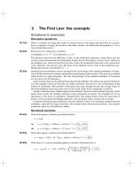
The vapour pressure of ice at −5◦ C is 3.9 × 10−3 atm, or 3 Torr. Therefore, the frost will sublime.
A partial pressure of 3 Torr or more will ensure that the frost remains.

E6.11(b)

(a) According to Trouton’s rule (Section 4.3, eqn 4.16)
vap H

= (85 J K−1 mol−1 ) × Tb = (85 J K−1 mol−1 ) × (342.2 K) = 29.1 kJ mol−1

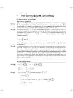
Solid

Liquid

Pressure

c

b
Critical
point

Start
d

a
Gas

Temperature

Figure 6.1


INSTRUCTOR’S MANUAL

90

(b) Use the Clausius–Clapeyron equation [Exercise 6.11(a)]
p2

p1

ln

vap H

=

R

×

1
1
−
T1
T2

At T2 = 342.2 K, p2 = 1.000 atm; thus at 25◦ C
29.1 × 103 J mol−1
8.314 J K−1 mol−1

ln p1 = −

×

1
1
−
298.2 K 342.2 K

= −1.509

×

1
1
−
333.2 K 342.2 K

= −0.276

p1 = 0.22 atm = 168 Torr
At 60◦ C,
29.1 × 103 J mol−1
8.314 J K−1 mol−1

ln p1 = −

p1 = 0.76 atm = 576 Torr
E6.12(b)

T = Tf (10 MPa) − Tf (0.1 MPa) =

Tf pM
fus H

1
ρ

= 6.01 kJ mol−1

fus H

(273.15 K) × (9.9 × 106 Pa) × (18 × 10−3 kg mol−1 )
6.01 × 103 J mol−1

T =

1
1
−
2
−3
9.98 × 10 kg m
9.15 × 102 kg m−3
= −0.74 K
×

Tf (10 MPa) = 273.15 K − 0.74 K = 272.41 K
E6.13(b)

vap H

=

vap U

+

vap (pV )

vap H

= 43.5 kJ mol−1

vap (pV )

= p vap V = p(Vgas − Vliq ) = pVgas = RT [per mole, perfect gas]

vap (pV )

= (8.314 J K−1 mol−1 ) × (352 K) = 2927 J mol−1

Fraction =

vap (pV )
vap H

=

2.927 kJ mol−1
43.5 kJ mol−1

= 6.73 × 10−2 = 6.73 per cent
E6.14(b)

Vm =

M

18.02 g mol−1
= 1.803 × 10−5 m3 mol−1
=
ρ
999.4 × 103 g m−3

2γ Vm
2(7.275 × 10−2 N m−1 ) × (1.803 × 10−5 m3 mol−1 )
=
rRT
(20.0 × 10−9 m) × (8.314 J K −1 mol−1 ) × (308.2 K)
= 5.119 × 10−2
p = (5.623 kPa)e0.05119 = 5.92 kPa


PHYSICAL TRANSFORMATIONS OF PURE SUBSTANCES

E6.15(b)

91

γ = 21 ρghr = 21 (0.9956 g cm−3 ) × (9.807 m s−2 ) × (9.11 × 10−2 m)
× (0.16 × 10−3 m) ×

1000 kg m−3
g cm−3

= 7.12 × 10−2 N m−1
E6.16(b)

pin − pout =

2γ
2(22.39 × 10−3 N m−1 )
=
r
(220 × 10−9 m)
= 2.04 × 105 N m−2 = 2.04 × 105 Pa

Solutions to problems
Solutions to numerical problems
P6.3

(a)

(b)

dp
=
dT

vap S

=

vap H

[6.6, Clapeyron equation]
Tb vap V
14.4 × 103 J mol−1

= + 5.56 kPa K−1
=
(180 K) × (14.5 × 10−3 − 1.15 × 10−4 ) m3 mol−1
vap V

dp
dp
vap H
× p 11, with d ln p =
=
2
p
dT
RT
3
−1
(14.4 × 10 J mol ) × (1.013 × 105 Pa)
=
= + 5.42 kPa K −1
(8.314 J K−1 mol−1 ) × (180 K)2
The percentage error is 2.5 per cent

P6.5

(a)

∂µ(l)
−
∂p T

1
∂µ(s)
= Vm (l) − Vm (s)[6.13] = M
ρ
∂p T
1
1
−1
−
= (18.02 g mol ) ×
−3
1.000 g cm
0.917 g cm−3
= −1.63 cm3 mol−1

(b)

∂µ(g)
−
∂p T

∂µ(l)
= Vm (g) − Vm (l)
∂p T
= (18.02 g mol−1 ) ×

1
1
−
0.598 g L−1

0.958 × 103 g L−1

= + 30.1 L mol−1
At 1.0 atm and 100◦ C , µ(l) = µ(g); therefore, at 1.2 atm and 100◦ C µ(g)−µ(l) ≈
(as in Problem 6.4)

P6.7

(30.1 × 10−3 m3 mol−1 ) × (0.2) × (1.013 × 105 Pa) ≈ + 0.6 kJ mol−1
Since µ(g) > µ(l), the gas tends to condense into a liquid.
pH2 O V
The amount (moles) of water evaporated is ng =
RT
The heat leaving the water is q = n vap H
The temperature change of the water is

T =

−q
, n = amount of liquid water
nCp,m

Vvap p =


INSTRUCTOR’S MANUAL

92

T =

Therefore,

−pH2 O V vap H
RT nCp,m
−(23.8 Torr) × (50.0 L) × (44.0 × 103 J mol−1 )

=

g
(62.364 L Torr K−1 mol−1 ) × (298.15 K) × (75.5 J K −1 mol−1 ) × 18.02250
g mol−1
= −2.7 K

The final temperature will be about 22◦ C
P6.9

(a) Follow the procedure in Problem 6.8, but note that Tb = 227.5◦ C is obvious from the data.
(b) Draw up the following table
θ/◦ C
T /K
1000 K/T
ln p/Torr

57.4
330.6
3.02
0.00

100.4

373.6
2.68
2.30

133.0
406.2
2.46
3.69

157.3
430.5
2.32
4.61

203.5
476.7
2.10
5.99

227.5
500.7
2.00
6.63

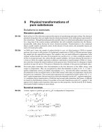
The points are plotted in Fig. 6.2. The slope is −6.4 × 103 K, so
implying that

= +53 kJ mol−1

vap H

− vap H
= −6.4 × 103 K,
R

6

4

2

0
2.0

2.2

2.4

2.6

2.8

3.0

Figure 6.2
P6.11

(a) The phase diagram is shown in Fig. 6.3.
2
Liquid

0
–2

Solid

Liquid–Vapour
Solid–Liquid

–4

Vapour

–6
–8
0

100

200

300

400

500

600

Figure 6.3

PHYSICAL TRANSFORMATIONS OF PURE SUBSTANCES

93

(b) The standard melting point is the temperature at which solid and liquid are in equilibrium at
1 bar. That temperature can be found by solving the equation of the solid–liquid coexistence
curve for the temperature
1 = p3 /bar + 1000(5.60 + 11.727x)x,
So 11 727x 2 + 5600x + (4.362 × 10−7 − 1) = 0
The quadratic formula yields
727)
−1 ± 1 + 4(11
−5600 ± {(5600)2 − 4(11 727) × (−1)}1/2
56002
x=
=
2(11 727)
2 11727
5600

1/2

The square root is rewritten to make it clear that the square root is of the form {1 + a}1/2 , with
a
1; thus the numerator is approximately −1 + (1 + 21 a) = 21 a, and the whole expression
reduces to
x ≈ 1/5600 = 1.79 × 10−4
Thus, the melting point is

T = (1 + x)T3 = (1.000179) × (178.15 K) = 178.18 K
(c) The standard boiling point is the temperature at which the liquid and vapour are in equilibrium
at 1 bar. That temperature can be found by solving the equation of the liquid–vapour coexistence
curve for the temperature. This equation is too complicated to solve analytically, but not difficult
to solve numerically with a spreadsheet. The calculated answer is T = 383.6 K
(d) The slope of the liquid–vapour coexistence curve is given by
dp
vap H
=
dT
T vap V −−

so

vap H

−−

= T vap V −−

dp
dT

The slope can be obtained by differentiating the equation for the coexistence curve.
dp
d ln p
d ln p dy
=p
=p
dT

dT
dy dT
dp
=
dT

10.418
− 15.996 + 2(14.015)y − 3(5.0120)y 2 − (1.70) × (4.7224) × (1 − y)0.70
y2
p
×
Tc
At the boiling point, y = 0.6458, so
dp
= 2.851 × 10−2 bar K−1 = 2.851 kPa K−1
dT
and
P6.12

vap H

−−

= (383.6 K) ×

(30.3 − 0.12) L mol−1
× (2.851 kPa K −1 ) = 33.0 kJ mol−1
1000 L m−3

The slope of the solid–vapour coexistence curve is given by

−−
dp
sub H
=
dT
T sub V −−

so

sub H

−−

= T sub V −−

dp
dT

The slope can be obtained by differentiating the coexistence curve graphically (Fig. 6.4).


INSTRUCTOR’S MANUAL

94

60
50
40
30
20

10
144

146

148

150

152

154

156

Figure 6.4

dp
= 4.41 Pa K−1
dT
according to the exponential best fit of the data. The change in volume is the volume of the vapour
Vm =

RT
(8.3145 J K−1 mol−1 ) × (150 K)
=
= 47.8 m3
p
26.1 Pa

So
sub H

−−

= (150 K) × (47.8 m3 ) × (4.41 Pa K −1 ) = 3.16 × 104 J mol−1 = 31.6 kJ mol−1

Solutions to theoretical problems
P6.14

P6.16

∂Gβ
∂ G
∂Gα
=
−
= Vβ − V α
∂p T
∂p T
∂p T
Therefore, if Vβ = Vα , G is independent of pressure. In general, Vβ = Vα , so that
though small, since Vβ − Vα is small.
pV
Amount of gas bubbled through liquid =
RT
(p = initial pressure of gas and emerging gaseous mixture)
m
Amount of vapour carried away =
M

Mole fraction of vapour in gaseous mixture =

Partial pressure of vapour = p =

m
M

m
M

+

pV
RT

m
M

G is nonzero,

m
M

pV
+ RT

×p =

p PmRT
VM

mRT
PVM

+1

=

mP A
,
mA + 1

A=

RT
PVM

For geraniol, M = 154.2 g mol−1 , T = 383 K, V = 5.00 L, p = 1.00 atm, and m = 0.32 g, so
A=

(8.206 × 10−2 L atm K−1 mol−1 ) × (383 K)
= 40.76 kg−1
(1.00 atm) × (5.00 L) × (154.2 × 10−3 kg mol−1 )

Therefore
p=

(0.32 × 10−3 kg) × (760 Torr) × (40.76 kg−1 )
= 9.8 Torr
(0.32 × 10−3 kg) × (40.76 kg−1 ) + 1

PHYSICAL TRANSFORMATIONS OF PURE SUBSTANCES

P6.17

p = p0 e−Mgh/RT [Box 1.1]
vap H
×
p = p∗ e−χ χ =
R

95

1
1
− ∗
T
T

[6.12]

Let T ∗ = Tb the normal boiling point; then p ∗ = 1 atm. Let T = Th , the boiling point at the
altitude h. Take p0 = 1 atm. Boiling occurs when the vapour (p) is equal to the ambient pressure,
that is, when p(T ) = p(h), and when this is so, T = Th . Therefore, since p0 = p∗ , p(T ) = p(h)
implies that
e−Mgh/RT = exp −

It follows that

vap H

R

×

1
1
−
Th
Tb

1
1
Mgh
=
+
Th
Tb
T vap H

where T is the ambient temperature and M the molar mass of the air. For water at 3000 m, using
M = 29 g mol−1
1
1
(29 × 10−3 kg mol−1 ) × (9.81 m s−2 ) × (3.000 × 103 m)
=
+
Th
373 K
(293 K) × (40.7 × 103 J mol−1 )

1
1
=
+
373 K 1.397 × 104 K
Hence, Th = 363 K (90◦ C)
P6.20

Sm = Sm (T , p)
∂Sm
dT +
dSm =
∂T p

∂Sm
dp
∂p T

Cp,m
∂Sm
=
[Problem 5.7]
∂T p
T

∂Vm
∂Sm
=−
[Maxwell relation]
∂p T

∂T p

∂Vm
dp
∂T p
∂q
∂p
Hm
= Cp,m − T Vm α
= Cp,m − αVm ×
[6.7]
CS =
∂T s
∂T s
Vm
−−
C(graphite)
C(diamond)
= 2.8678 kJ mol−1 at TC.
rG
dqrev = T dSm = Cp,m dT − T

P6.22

We want the pressure at which r G = 0; above that pressure the reaction will be spontaneous.
Equation 5.10 determines the rate of change of r G with p at constant T .
(1)

(2)

∂ rG
= r V = (VD − VG )M
∂p
T
where M is the molar mas of carbon; VD and VG are the specific volumes of diamond and
graphite, respectively.
−
C, p) may be expanded in a Taylor series around the pressure p −
C.
= 100 kPa at T
r G(T
C,
r G(T

p) =

rG

+

1
2

∂ r G−− (TC, p −− )
(p − p −− )
∂p
T
∂ 2 r G−− (TC, p −− )
(p − p −− )2 + θ(p − p −− )3
∂p 2

−− C
(T,

p −− ) +

T


INSTRUCTOR’S MANUAL

96

We will neglect the third and higher-order terms; the derivative of the first-order term can be
calculated with eqn 1. An expression for the derivative of the second-order term can be derived
with eqn 1.
(3)

∂VG
∂VD
M = {VG κT (G) − VD κT (D)}M [3.13]
−
∂p T
∂p T
T
Calculating the derivatives of eqns 1 and 2 at TC and p −−
∂2 rG
∂p 2

=

(4)

∂ r G(TC, p −− )
= (0.284 − 0.444) ×
∂p
T

(5)

∂ 2 r G(TC, p −− )
∂p 2

cm3
g

×

12.01 g
mol

= −1.92 cm3 mol−1

= {0.444(3.04 × 10−8 ) − 0.284(0.187 × 10−8 )}
T

×

cm3 kPa−1
g

×

12.01 g
mol

= 1.56 × 10−7 cm3 (kPa)−1 mol−1
It is convenient to convert the value of r G−− to the units cm3 kPa mol−1
8.315 × 10−2 L bar K−1 mol−1
103 cm3
−−
×
= 2.8678 kJ mol−1
rG
L
8.315 J K−1 mol−1
(6)

×

105 Pa
bar

= 2.8678 × 106 cm3 kPa mol−1
Setting χ = p − p −− , eqns 2 and 3–6 give
2.8678 × 106 cm3 kPa mol−1 − (1.92 cm3 mol−1 )χ + (7.80 × 10−8 cm3 kPa−1 mol−1 )χ 2 = 0
when r G(TC, p) = 0. One real root of this equation is
rG

−−

χ = 1.60 × 106 kPa = p − p −− or
p = 1.60 × 106 kPa − 102 kPa
= 1.60 × 106 kPa = 1.60 × 104 bar
Above this pressure the reaction is spontaneous. The other real root is much higher: 2.3×107 kPa.
Question. What interpretation might you give to the other real root?