Instructor solution manual to accompany physical chemistry 7th ed by peter atkins chap07

7

Simple mixtures

Solutions to exercises
Discussion questions
E7.1(b)

For a component in an ideal solution, Raoult’s law is: p = xp ∗ . For real solutions, the activity, a,
replaces the mole fraction, x, and Raoult’s law becomes p = ap ∗ .

E7.2(b)

All the colligative properties are a result of the lowering of the chemical potential of the solvent
due to the presence of the solute. This reduction takes the form µA = µA ∗ + RT ln xA or µA =
µA ∗ + RT ln aA , depending on whether or not the solution can be considered ideal. The lowering of
the chemical potential results in a freezing point depression and a boiling point elevation as illustrated
in Fig. 7.20 of the text. Both of these effects can be explained by the lowering of the vapour pressure
of the solvent in solution due to the presence of the solute. The solute molecules get in the way of
the solvent molecules, reducing their escaping tendency.

E7.3(b)

The activity of a solute is that property which determines how the chemical potential of the solute
varies from its value in a specified reference state. This is seen from the relation µ = µ−− + RT ln a,
where µ−− is the value of the chemical potential in the reference state. The reference state is either the
hypothetical state where the pure solute obeys Henry’s law (if the solute is volatile) or the hypothetical
state where the solute at unit molality obeys Henry’s law (if the solute is involatile). The activity of
the solute can then be defined as that physical property which makes the above relation true. It can
be interpreted as an effective concentration.

Numerical exercises
E7.4(b)

Total volume V = nA VA + nB VB = n(xA VA + xB VB )
Total mass m = nA MA + nB MB
= n(xA MA + (1 − xA )MB )
m
=n
xA MA + (1 − xA )MB

where n = nA + nB

1.000 kg(103 g/kg)
= 4.6701¯ mol
(0.3713) × (241.1 g/mol) + (1 − 0.3713) × (198.2 g/mol)
V = n(xA VA + xB VB )
= (4.6701¯ mol) × [(0.3713) × (188.2 cm3 mol−1 ) + (1 − 0.3713) × (176.14 cm3 mol−1 )]
n=

= 843.5 cm3
E7.5(b)

Let A denote water and B ethanol. The total volume of the solution is V = nA VA + nB VB
We know VB ; we need to determine nA and nB in order to solve for VA .
Assume we have 100 cm3 of solution; then the mass is
m = ρV = (0.9687 g cm−3 ) × (100 cm3 ) = 96.87 g
of which (0.20) × (96.87 g) = 19.374 g is ethanol and (0.80) × (96.87 g) = 77.496 g is water.
77.496 g
= 4.30 mol H2 O
18.02 g mol−1

19.374 g
nB =
= 0.4205 mol ethanol
46.07 g mol−1
nA =


INSTRUCTOR’S MANUAL

98

100 cm3 − (0.4205 mol) × (52.2 cm3 mol−1 )
V − n B VB
= 18.15 cm3
= VA =
nA
4.30¯ mol
= 18 cm3
E7.6(b)

Check that pB /xB = a constant (KB )
xB
(pB /xB )/kPa

0.010
8.2 × 103

0.015
8.1 × 103

0.020
8.3 × 103

KB = p/x, average value is 8.2 × 103 kPa
E7.7(b)

In exercise 7.6(b), the Henry’s law constant was determined for concentrations expressed in mole
fractions. Thus the concentration in molality must be converted to mole fraction.
m(A) = 1000 g, corresponding to
1000 g
n(A) =
= 13.50¯ mol
74.1 g mol−1

n(B) = 0.25 mol

Therefore,
0.25 mol
= 0.0182¯
0.25 mol + 13.50¯ mol

xB =

using KB = 8.2 × 103 kPa [exercise 7.6(b)]
p = 0.0182¯ × 8.2 × 103 kPa = 1.5 × 102 kPa

E7.8(b)

Kf =

RT ∗2 M
8.314 J K−1 mol−1 × (354 K)2 × 0.12818 kg mol−1
=
18.80 × 103 J mol−1
fus H
= 7.1 K kg mol−1

Kb =

RT ∗2 M
8.314 J K−1 mol−1 × (490.9 K)2 × 0.12818 kg mol−1
=
51.51 × 103 J mol−1
vap H
= 4.99 K kg mol−1

E7.9(b)

We assume that the solvent, 2-propanol, is ideal and obeys Raoult’s law.
xA (solvent) = p/p ∗ =

49.62
= 0.9924
50.00

MA (C3 H8 O) = 60.096 g mol−1
250 g
= 4.1600 mol
60.096 g mol−1
nA

nA
xA =
nA + n B =
nA + n B
xA
nA =


SIMPLE MIXTURES

99

nB = nA

1
−1
xA

= 4.1600 mol

8.69 g
= 273¯ g mol−1 = 270 g mol−1
3.186 × 10−2 mol

MB =
E7.10(b)

1
− 1 = 3.186 × 10−2 mol
0.9924

Kf = 6.94 for naphthalene
mass of B
nB

MB =

nB = mass of naphthalene · bB
bB =

T
Kf

so

MB =

(mass of B) × Kf
(mass of naphthalene) ×

T

(5.00 g) × (6.94 K kg mol−1 )
= 178 g mol−1
(0.250 kg) × (0.780 K)
nB
nB
=
T = Kf bB and bB =
mass of water

Vρ

MB =
E7.11(b)

ρ = 103 kg m−3
nB =

V
RT

T =

(density of solution ≈ density of water)
T = Kf

RT ρ

Kf = 1.86 K mol−1 kg

(1.86 K kg mol−1 ) × (99 × 103 Pa)
= 7.7 × 10−2 K
(8.314 J K−1 mol−1 ) × (288 K) × (103 kg m−3 )

Tf = −0.077◦ C
E7.12(b)

mix G

= nRT (xA ln xA + xB ln xB )

nAr = nNe ,
mix G

xAr = xNe = 0.5,

n = nAr + nNe =

= pV 21 ln 21 + 21 ln 21 = −pV ln 2
= −(100 × 103 Pa) × (0.250 L)
= −17.3 Pa m3 = −17.3 J

E7.13(b)

mix G

pV
RT

= nRT

xJ ln xJ [7.18]
J

1 m3
ln 2
103 L
17.3 J
− mix G
=

= 6.34 × 10−2 J K−1
T
273 K
− mix G
xJ ln xJ [7.19] =
mix S = −nR
T
J
mix S

=

n = 1.00 mol + 1.00 mol = 2.00 mol
x(Hex) = x(Hep) = 0.500
Therefore,
mix G

= (2.00 mol) × (8.314 J K −1 mol−1 ) × (298 K) × (0.500 ln 0.500 + 0.500 ln 0.500)
= −3.43 kJ


INSTRUCTOR’S MANUAL

100

+3.43 kJ
= +11.5 J K−1
298 K
mix H for an ideal solution is zero as it is for a solution of perfect gases [7.20]. It can be demonstrated
from

mix S

mix H

E7.14(b)

=

=

mix G + T

mix S

= (−3.43 × 103 J) + (298 K) × (11.5 J K −1 ) = 0

Benzene and ethylbenzene form nearly ideal solutions, so
mix S

= −nR(xA ln xA + xB ln xB )
mix S, differentiate with respect to xA

To find maximum
is zero.

and find value of xA at which the derivative

Note that xB = 1 − xA so
mix S

use

= −nR(xA ln xA + (1 − xA ) ln(1 − xA ))

1
d ln x
=
x
dx
xA
d
( mix S) = −nR(ln xA + 1 − ln(1 − xA ) − 1) = −nR ln
dx
1 − xA
=0

when xA = 21

Thus the maximum entropy of mixing is attained by mixing equal molar amounts of two components.
mB /MB
nB
= 1 =
nE
mE /ME

mE
ME
106.169
= 1.3591
=

=
78.115
mB
MB

mB
= 0.7358
mE
E7.15(b)

Assume Henry’s law [7.26] applies; therefore, with K(N2 ) = 6.51 × 107 Torr and K(O2 ) = 3.30 ×
107 Torr, as in Exercise 7.14, the amount of dissolved gas in 1 kg of water is
n(N2 ) =

103 g
18.02 g mol−1

×

p(N2 )
6.51 × 107 Torr

= (8.52 × 10−7 mol) × (p/Torr)

For p(N2 ) = xp and p = 760 Torr
n(N2 ) = (8.52 × 10−7 mol) × (x) × (760) = x(6.48 × 10−4 mol)
and, with x = 0.78
n(N2 ) = (0.78) × (6.48 × 10−4 mol) = 5.1 × 10−4 mol = 0.51 mmol
The molality of the solution is therefore approximately 0.51 mmol kg−1 in N2 . Similarly, for oxygen,
n(O2 ) =

103 g
18.02 g mol−1

×

p(O2 )
3.30 × 107 Torr

= (1.68 × 10−6 mol) × (p/Torr)

For p(O2 ) = xp and p = 760 Torr
n(O2 ) = (1.68 × 10−6 mol) × (x) × (760) = x(1.28 mmol)
and when x = 0.21, n(O2 ) ≈ 0.27 mmol. Hence the solution will be 0.27 mmol kg−1 in O2 .


SIMPLE MIXTURES

E7.16(b)

101

Use n(CO2 ) = (4.4 × 10−5 mol) × (p/Torr), p = 2.0(760 Torr) = 1520 Torr
n(CO2 ) = (4.4 × 10−5 mol) × (1520) = 0.067 mol
The molality will be about 0.067 mol kg−1 and, since molalities and molar concentration for dilute
aqueous solutions are approximately equal, the molar concentration is about 0.067 mol L−1

E7.17(b)

M(glucose) = 180.16 g mol−1

T = Kf bB

Kf = 1.86 K kg mol−1

T = (1.86 K kg mol−1 ) ×

10 g/180.16 g mol−1
0.200 kg

= 0.52 K

Freezing point will be 0◦ C − 0.52◦ C = −0.52◦ C
E7.18(b)

The procedure here is identical to Exercise 7.18(a).
ln xB =
=

fus H

R

×

5.2 × 103 J mol−1
8.314 J K−1 mol−1

¯
= −0.0886,
xB =

1
1
−
∗
T
T

[7.39; B, the solute, is lead]
×

1
1
−
600 K 553 K

implying that xB = 0.92

n(Pb)
,
n(Pb) + n(Bi)

implying that n(Pb) =

xB n(Bi)
1 − xB

1000 g
= 4.785 mol
208.98 g mol−1

Hence, the amount of lead that dissolves in 1 kg of bismuth is

For 1 kg of bismuth, n(Bi) =

n(Pb) =

(0.92) × (4.785 mol)
= 55 mol,
1 − 0.92

11 kg

or

Comment. It is highly unlikely that a solution of 11 kg of lead and 1 kg of bismuth could in any
sense be considered ideal. The assumptions upon which eqn 7.39 is based are not likely to apply. The
answer above must then be considered an order of magnitude result only.
E7.19(b)

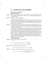
Proceed as in Exercise 7.19(a). The data are plotted in Fig. 7.1, and the slope of the line is 1.78 cm/
(mg cm−3 ) = 1.78 cm/(g L−1 ) = 1.78 × 10−2 m4 kg−1 .
12

10

8

6
3

4

5

6

7

Figure 7.1


INSTRUCTOR’S MANUAL

102

Therefore,
(8.314 J K−1 mol−1 ) × (293.15 K)
= 14.0 kg mol−1
(1.000 × 103 kg m−3 ) × (9.81 m s−2 ) × (1.78 × 10−2 m4 kg−1 )

M=
E7.20(b)

Let A = water and B = solute.
pA
0.02239 atm
= 0.9701
[42] =
∗
pA

0.02308 atm
nA
aA
and xA =
γA =
xA
nA + n B
0.122 kg
0.920 kg
= 0.506 mol
nA =
= 51.05¯ mol
nB =
−1
0.01802 kg mol
0.241 kg mol−1
51.05¯
0.9701
xA =
= 0.990
γA =
= 0.980
51.05 + 0.506
0.990

aA =

E7.21(b)

B = Benzene

µB (l) = µ∗B (l) + RT ln xB [7.50, ideal solution]

RT ln xB = (8.314 J K−1 mol−1 ) × (353.3 K) × (ln 0.30) = −3536¯ J mol−1
Thus, its chemical potential is lowered by this amount.
∗
∗
[42] = γB xB pB
= (0.93) × (0.30) × (760 Torr) = 212 Torr
pB = aB pB

E7.22(b)

Question. What is the lowering of the chemical potential in the nonideal solution with γ = 0.93?
pA
pA
=
yA =
= 0.314
pA + p B
760 Torr
pA = (760 Torr) × (0.314) = 238.64 Torr
pB = 760 Torr − 238.64 Torr = 521.36 Torr
pA
238.64 Torr
aA = ∗ =
1 atm
pA
(73.0 × 103 Pa) ×
× 760 Torr

101 325 Pa

aB =

= 0.436

atm

pB
521.36 Torr
∗ =
atm
760 Torr
pB
3
(92.1 × 10 Pa) × 1011 325
atm
Pa ×

= 0.755

aA
0.436
=
= 1.98
xA
0.220
aB
0.755
γB =

= 0.968
=
xB
0.780
γA =

Solutions to problems
Solutions to numerical problems
P7.3

Vsalt =

∂V
mol−1 [Problem 7.2]
∂b H2 O

= 69.38(b − 0.070) cm3 mol−1

with b ≡ b/(mol kg−1 )

Therefore, at b = 0.050 mol kg−1 , Vsalt = −1.4 cm3 mol−1


SIMPLE MIXTURES

103

The total volume at this molality is
V = (1001.21) + (34.69) × (0.02)2 cm3 = 1001.22 cm3
Hence, as in Problem 7.2,

V (H2 O) =

(1001.22 cm3 ) − (0.050 mol) × (−1.4 cm3 mol−1 )
= 18.04 cm3 mol−1
55.49 mol

Question. What meaning can be ascribed to a negative partial molar volume?
P7.5

Let E denote ethanol and W denote water; then
V = nE VE + nW VW [7.3]
For a 50 per cent mixture by mass, mE = mW , implying that
nE ME = nW MW ,
Hence, V = nE VE +
which solves to nE =
Furthermore, xE =

or

nW =

n E M E VW
MW
V
VE +

ME VW
MW

nE ME

MW

, nW =

ME V
VE M W + M E V W

nE
1
=
ME
nE + n W
1+ M
W

Since ME = 46.07 g mol−1 and MW = 18.02 g mol−1 ,
xE = 0.2811,

ME
= 2.557. Therefore
MW

xW = 1 − xE = 0.7189

At this composition
VE = 56.0 cm3 mol−1
Therefore, nE =

VW = 17.5 cm3 mol−1 [Fig.7.1 of the text]
100 cm3

(56.0 cm3 mol−1 ) + (2.557) × (17.5 cm3 mol−1 )

= 0.993 mol

nW = (2.557) × (0.993 mol) = 2.54 mol
The fact that these amounts correspond to a mixture containing 50 per cent by mass of both components
is easily checked as follows
mE = nE ME = (0.993 mol) × (46.07 g mol−1 ) = 45.7 g ethanol
mW = nW MW = (2.54 mol) × (18.02 g mol−1 ) = 45.7 g water
At 20◦ C the densities of ethanol and water are, ρE = 0.789 g cm−3 , ρW = 0.997 g cm−3 . Hence,
VE =

mE
45.7 g
=
= 57.9 cm3 of ethanol
ρE
0.789 g cm−3

VW =

mW
45.7 g
=
= 45.8 cm3 of water
ρW
0.997 g cm−3

INSTRUCTOR’S MANUAL

104

The change in volume upon adding a small amount of ethanol can be approximated by
V =

dV ≈

VE dnE ≈ VE

nE

where we have assumed that both VE and VW are constant over this small range of nE . Hence
(1.00 cm3 ) × (0.789 g cm−3 )
(46.07 g mol−1 )

V ≈ (56.0 cm3 mol−1 ) ×

P7.7

T
0.0703 K
= 0.0378 mol kg−1
=
Kf
1.86 K/(mol kg−1 )

Since the solution molality is nominally 0.0096 mol kg−1 in Th(NO3 )4 , each formula unit supplies
0.0378

≈ 4 ions. (More careful data, as described in the original reference gives ν ≈ 5 to 6.)
0.0096
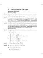
The data are plotted in Figure 7.2. The regions where the vapor pressure curves show approximate
straight lines are denoted R for Raoult and H for Henry. A and B denote acetic acid and benzene
respectively.
300
Extrapolate
for KB

R

Henry

200
B
p / Torr

P7.9

mB =

= +0.96 cm3

Raoult

100
Henry

A

H

Raoult
0

0

0.2

0.4

0.6
xA

R

H
0.8

1.0

Figure 7.2

pA
pB
∗ and γB = x p ∗ for the Raoult’s law activity
xA p A
B B
pB
coefficients and γB =

for the activity coefficient of benzene on a Henry’s law basis, with K
xB K
∗
∗
determined by extrapolation. We use pA
= 55 Torr, pB
= 264 Torr and KB∗ = 600 Torr to draw up
As in Problem 7.8, we need to form γA =


SIMPLE MIXTURES

105

the following table:
xA
pA /Torr
pB /Torr
aA (R)
aB (R)
γA (R)
γB (R)
aB (H)
γB (H)

0
0
264
0
1.00

—
1.00
0.44
0.44

0.2
20
228
0.36
0.86
1.82
1.08
0.38
0.48

0.4
30
190
0.55
0.72
1.36
1.20
0.32
0.53

0.6
38
150
0.69
0.57

1.15
1.42
0.25
0.63

0.8
50
93
0.91
0.35
1.14
1.76
0.16
0.78

1.0
55
0
1.00[pA /pA∗ ]
0[pB /pB∗ ]
1.00[pA /xA pA∗ ]
—[pB /xB pB∗ ]
0[pB /KB ]
1.00[pB /xB KB ]

GE is defined as [Section 7.4]:
GE =

mix G(actual) −

mix G(ideal)

= nRT (xA ln aA + xB ln aB ) − nRT (xA ln xA + xB ln xB )

and with a = γ x
GE = nRT (xA ln γA + xA ln γB ).
For n = 1, we can draw up the following table from the information above and RT = 2.69 kJ mol−1 :
xA
xA ln γA
xB ln γB
GE /(kJ mol−1 )

P7.11

0
0
0
0

0.2
0.12
0.06
0.48

0.4
0.12
0.11
0.62

0.6

0.08
0.14
0.59

0.8
0.10
0.11
0.56

1.0
0
0
0

(a) The volume of an ideal mixture is
Videal = n1 Vm,1 + n2 Vm,2
so the volume of a real mixture is
V = Videal + V E
We have an expression for excess molar volume in terms of mole fractions. To compute partial
molar volumes, we need an expression for the actual excess volume as a function of moles
V E = (n1 + n2 )VmE =

n 1 n2
n1 + n 2

a0 +

a1 (n1 − n2 )
n1 + n 2

n1 n2
a1 (n1 − n2 )
a0 +
n1 + n 2
n1 + n 2
The partial molar volume of propionic acid is

so V = n1 Vm,1 + n2 Vm,2 +

V1 =

a0 n22
a1 (3n1 − n2 )n22
∂V
= Vm,1 +
+
∂n1 p,T ,n2
(n1 + n2 )2
(n1 + n2 )3

V1 = Vm,1 + a0 x22 + a1 (3x1 − x2 )x22
That of oxane is
V2 = Vm,2 + a0 x12 + a1 (x1 − 3x2 )x12


INSTRUCTOR’S MANUAL

106

(b) We need the molar volumes of the pure liquids

Vm,1 =

M1
74.08 g mol−1
=
= 76.23 cm3 mol−1
ρ1
0.97174 g cm−3

86.13 g mol−1
= 99.69 cm3 mol−1
0.86398 g cm−3
In an equimolar mixture, the partial molar volume of propionic acid is
and Vm,2 =

V1 = 76.23 + (−2.4697) × (0.500)2 + (0.0608) × [3(0.5) − 0.5] × (0.5)2 cm3 mol−1
= 75.63 cm3 mol−1
and that of oxane is
V2 = 99.69 + (−2.4697) × (0.500)2 + (0.0608) × [0.5 − 3(0.5)] × (0.5)2 cm3 mol−1
= 99.06 cm3 mol−1
P7.13

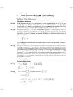
Henry’s law constant is the slope of a plot of pB versus xB in the limit of zero xB (Fig. 7.3). The
partial pressures of CO2 are almost but not quite equal to the total pressures reported above
pCO2 = pyCO2 = p(1 − ycyc )
Linear regression of the low-pressure points gives KH = 371 bar
80

60

40

20

0
0.0

0.1

0.2

0.3

Figure 7.3
The activity of a solute is
aB =

pB
= xB γB
KH

so the activity coefficient is
γB =

pB
yB p
=
xB K H
xB K H

SIMPLE MIXTURES

107

where the last equality applies Dalton’s law of partial pressures to the vapour phase. A spreadsheet
applied this equation to the above data to yield
p/bar
10.0
20.0
30.0
40.0
60.0
80.0

P7.16

ycyc
0.0267
0.0149
0.0112
0.009 47
0.008 35
0.009 21

xcyc
0.9741
0.9464
0.9204
0.892

0.836
0.773

γCO2
1.01
0.99
1.00
0.99
0.98
0.94

GE = RT x(1 − x){0.4857 − 0.1077(2x − 1) + 0.0191(2x − 1)2 }
with x = 0.25 gives GE = 0.1021RT . Therefore, since
mix G(actual)
mix G

=

mix G(ideal) + nG

E

= nRT (xA ln xA + xB ln xB ) + nGE = nRT (0.25 ln 0.25 + 0.75 ln 0.75) + nGE
= −0.562nRT + 0.1021nRT = −0.460nRT

Since n = 4 mol and RT = (8.314 J K −1 mol−1 ) × (303.15 K) = 2.52 kJ mol−1 ,
mix G

= (−0.460) × (4 mol) × (2.52 kJ mol−1 ) = −4.6 kJ

Solutions to theoretical problems
P7.18

xA dµA + xB dµB = 0 [7.11, Gibbs–Duhem equation]
Therefore, after dividing through by dxA
xA

∂µA
+ xB
∂xA p,T

∂µB
=0
∂xA p,T

or, since dxB = −dxA , as xA + xB = 1
xA

∂µA
− xB
∂xA p,T

∂µB
=0
∂xB p,T

∂µA
=
∂ ln xA p,T

dx
∂µB
d ln x =
∂ ln xB p,T
x
f
∂ ln fA
Then, since µ = µ−− + RT ln −− ,
=
p
∂ ln xA p,T
∂ ln pA
∂ ln pB
On replacing f by p,
=
∂ ln xA p,T
∂ ln xB p,T
or,

∂ ln fB
∂ ln xB p,T

∗
If A satisfies Raoult’s law, we can write pA = xA pA
, which implies that
∗
∂ ln pA
∂ ln pA
∂ ln xA
=

+
=1+0
∂ ln xA p,T
∂ ln xA
∂ ln xA

∂ ln pB
=1
∂ ln xB p,T
∗
which is satisfied if pB = xB pB
(by integration, or inspection). Hence, if A satisfies Raoult’s law, so
does B.
Therefore,


INSTRUCTOR’S MANUAL

108

P7.20

ln xA =

− fus G
(Section 7.5 analogous to equation for ln xB used in derivation of eqn 7.39)
RT

d ln xA
1

d
=− ×
dT
R
dT
xA
1

d ln xA =

ln xA =

T

fus G

T
fus H dT
RT 2

T∗

=

− fus H
×
R

≈

fus H
RT 2
fus H

R

[Gibbs–Helmholtz equation]
T

dT
2
T∗ T

1
1
− ∗
T
T

The approximations ln xA ≈ −xB and T ≈ T ∗ then lead to eqns 33 and 36, as in the text.
P7.22

Retrace the argument leading to eqn 7.40 of the text. Exactly the same process applies with aA in
place of xA . At equilibrium
µ∗A (p) = µA (xA , p +

)

which implies that, with µ = µ∗ + RT ln a for a real solution,

p+

and hence that

p

p+

) + RT ln aA = µ∗A (p) +

µ∗A (p) = µ∗A (p +

p

Vm dp + RT ln aA

Vm dp = −RT ln aA

For an incompressible solution, the integral evaluates to

Vm , so

Vm = −RT ln aA

In terms of the osmotic coefficient φ (Problem 7.21)
Vm = rφRT

r=

xB

nB
=
xA
nA

φ=−

xA
1
ln aA = − ln aA
xB
r

For a dilute solution, nA Vm ≈ V
Hence,

V = nB φRT

and therefore, with [B] =

nB
V

= φ[B]RT

Solutions to applications
P7.24

By the van’t Hoff equation [7.40]
cRT

Π = [B]RT =
M
Division by the standard acceleration of free fall, g, gives
Π
c(R/g)T
=
8
M
(a) This expression may be written in the form
cR T
Π =
M
which has the same form as the van’t Hoff equation, but the unit of osmotic pressure (Π ) is now
force/area
(mass length)/(area time2 )
mass
=
=
2
area
length/time
length/time2


SIMPLE MIXTURES

109

This ratio can be specified in g cm−2 . Likewise, the constant of proportionality (R ) would have
the units of R/g

(mass length2 /time2 ) K−1 mol−1
energy K −1 mol−1
=
= mass length K −1 mol−1
2
2
length/time
length/time
This result may be specified in g cm K−1 mol−1
R =

8.314 51 J K−1 mol−1
R
=
g
9.806 65m s−2

= 0.847 844 kg m K−1 mol−1

103 g
kg

×

102 cm
m

R = 84 784.4 g cm K−1 mol−1
In the following we will drop the primes giving
cRT

Π=
M
and use the Π units of g cm−2 and the R units g cm K−1 mol−1 .
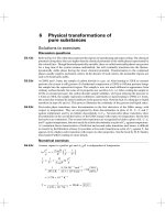
(b) By extrapolating the low concentration plot of /c versus c (Fig. 7.4 (a)) to c = 0 we find the
intercept 230 g cm−2 /g cm−3 . In this limit van’t Hoff equation is valid so
RT
RT
= intercept or M n =
intercept
Mn
(84 784.4 g cm K−1 mol−1 ) × (298.15 K)
Mn =
(230 g cm−2 )/(g cm−3 )
M n = 1.1 × 105 g mol

−1

500

450

400

350

300

250

200

0.000

0.010

0.020

0.030

0.040

Figure 7.4(a)


INSTRUCTOR’S MANUAL

110

(c) The plot of Π/c versus c for the full concentration range (Fig. 7.4(b)) is very nonlinear. We may
conclude that the solvent is good . This may be due to the nonpolar nature of both solvent and
solute.

7000

6000

5000

4000

3000

2000

1000

0
0.00

0.050

0.100

0.150

0.200

0.250

0.300

Figure 7.4(b)

(d) Π/c = (RT /M n )(1 + B c + C c2 )
Since RT /M n has been determined in part (b) by extrapolation to c = 0, it is best to determine
the second and third virial coefficients with the linear regression fit
(Π/c)/(RT /M n ) − 1
=B +C c
c
R = 0.9791
B = 21.4 cm3 g−1 ,

C = 211 cm6 g−2 ,

standard deviation = 2.4 cm3 g−1
standard deviation = 15 cm6 g−2

(e) Using 1/4 for g and neglecting terms beyond the second power, we may write
Π 1/2
=
c

RT 1/2
Mn

(1 + 21 B c)


SIMPLE MIXTURES

111

We can solve for B , then g(B )2 = C .


1/2



Π
c

RT
Mn



1/2 

− 1 = 21 B c

RT /M n has been determined above as 230 g cm−2 /g cm−3 . We may analytically solve for B
from one of the data points, say, /c = 430 g cm−2 /g cm−3 at c = 0.033 g cm−3 .
430 g cm−2 /g cm−3 1/2
− 1 = 21 B × (0.033 g cm−3 )
230 g cm−2 /g cm−3
2 × (1.367 − 1)
B =
= 22.2¯ cm3 g−1
0.033 g cm−3
C = g(B )2 = 0.25 × (22.2¯ cm3 g−1 )2 = 123¯ cm6 g−2
Better values of B and C can be obtained by plotting

Π

1/2

RT 1/2

c

Mn

against c. This plot

is shown in Fig. 7.4(c). The slope is 14.03 cm3 g−1 . B = 2 × slope = 28.0¯ cm3 g−1 C is then
196¯ cm6 g−2 The intercept of this plot should thereotically be 1.00, but it is in fact 0.916 with a
standard deviation of 0.066. The overall consistency of the values of the parameters confirms that g
is roughly 1/4 as assumed.
6.0

5.0

n

4.0

3.0

2.0

1.0

0.0
0.00

0.05

0.10

0.15

0.20

0.25

0.30

Figure 7.4(c)