Solutions fundamentals of futures and options markets 7e by hull chapter 19

CHAPTER 19
Volatility Smiles
Problem 19.8.
A stock price is currently $20. Tomorrow, news is expected to be announced that will either
increase the price by $5 or decrease the price by $5. What are the problems in using Black–
Scholes to value one-month options on the stock?
The probability distribution of the stock price in one month is not lognormal. Possibly it
consists of two lognormal distributions superimposed upon each other and is bimodal. Black–
Scholes is clearly inappropriate, because it assumes that the stock price at any future time is
lognormal.
Problem 19.9.
What volatility smile is likely to be observed for six-month options when the volatility is
uncertain and positively correlated to the stock price?
When the asset price is positively correlated with volatility, the volatility tends to increase as
the asset price increases, producing less heavy left tails and heavier right tails. Implied
volatility then increases with the strike price.
Problem 19.10.
What problems do you think would be encountered in testing a stock option pricing model
empirically?
There are a number of problems in testing an option pricing model empirically. These include
the problem of obtaining synchronous data on stock prices and option prices, the problem of
estimating the dividends that will be paid on the stock during the option’s life, the problem of
distinguishing between situations where the market is inefficient and situations where the
option pricing model is incorrect, and the problems of estimating stock price volatility.
Problem 19.11.
Suppose that a central bank’s policy is to allow an exchange rate to fluctuate between 0.97
and 1.03. What pattern of implied volatilities for options on the exchange rate would you
expect to see?
In this case the probability distribution of the exchange rate has a thin left tail and a thin right
tail relative to the lognormal distribution. We are in the opposite situation to that described
for foreign currencies in Section 19.1. Both out-of-the-money and in-the-money calls and

puts can be expected to have lower implied volatilities than at-the-money calls and puts. The
pattern of implied volatilities is likely to be similar to Figure 19.7.
Problem 19.12.
Option traders sometimes refer to deep-out-of-the-money options as being options on
volatility. Why do you think they do this?
A deep-out-of-the-money option has a low value. Decreases in its volatility reduce its value.


However, this reduction is small because the value can never go below zero. Increases in its
volatility, on the other hand, can lead to significant percentage increases in the value of the
option. The option does, therefore, have some of the same attributes as an option on volatility.
Problem 19.13.
A European call option on a certain stock has a strike price of $30, a time to maturity of one
year, and an implied volatility of 30%. A European put option on the same stock has a strike
price of $30, a time to maturity of one year, and an implied volatility of 33%. What is the
arbitrage opportunity open to a trader? Does the arbitrage work only when the lognormal
assumption underlying Black–Scholes–Merton holds? Explain the reasons for your answer
carefully.
As explained in the appendix to the chapter, put–call parity implies that European put and call
options have the same implied volatility. If a call option has an implied volatility of 30% and
a put option has an implied volatility of 33%, the call is priced too low relative to the put. The
correct trading strategy is to buy the call, sell the put and short the stock. This does not
depend on the lognormal assumption underlying Black–Scholes–Merton. Put–call parity is
true for any set of assumptions.
Problem 19.14.
Suppose that the result of a major lawsuit affecting a company is due to be announced
tomorrow. The company’s stock price is currently $60. If the ruling is favorable to the
company, the stock price is expected to jump to $75. If it is unfavorable, the stock is expected
to jump to $50. What is the risk-neutral probability of a favorable ruling? Assume that the
volatility of the company’s stock will be 25% for six months after the ruling if the ruling is

favorable and 40% if it is unfavorable. Use DerivaGem to calculate the relationship between
implied volatility and strike price for six-month European options on the company today. The
company does not pay dividends. Assume that the six-month risk-free rate is 6%. Consider
call options with strike prices of $30, $40, $50, $60, $70, and $80.
Suppose that p is the probability of a favorable ruling. The expected price of the company’s
stock tomorrow is
75 p  50(1  p )  50  25 p
This must be the price of the stock today. (We ignore the expected return to an investor over
one day.) Hence
50  25 p  60
or p  04 .
If the ruling is favorable, the volatility,  , will be 25%. Other option parameters are
S0  75 , r  006 , and T  05 . For a value of K equal to 50, DerivaGem gives the value of
a European call option price as 26.502.
If the ruling is unfavorable, the volatility,  will be 40% Other option parameters are
S0  50 , r  006 , and T  05 . For a value of K equal to 50, DerivaGem gives the value of
a European call option price as 6.310.
The value today of a European call option with a strike price today is the weighted average of
26.502 and 6.310 or:
04 �26502  06 �6310  14387
DerivaGem can be used to calculate the implied volatility when the option has this price. The
parameter values are S0  60 , K  50 , T  05 , r  006 and c  14387 . The implied


volatility is 47.76%.
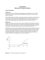
These calculations can be repeated for other strike prices. The results are shown in the table
below. The pattern of implied volatilities is shown in Figure S19.1.
Strike
Price
30

40
50
60
70
80

Figure S19.1

Call Price:
Favorable Outcome
45.887
36.182
26.502
17.171
9.334
4.159

Call Price:
Unfavorable Outcome
21.001
12.437
6.310
2.826
1.161
0.451

Weighted
Price
30.955
21.935

14.387
8.564
4.430
1.934

Implied Volatility
(%)
46.67
47.78
47.76
46.05
43.22
40.36

Implied Volatilities in Problem 19.14

Problem 19.15.
An exchange rate is currently 0.8000. The volatility of the exchange rate is quoted as 12%
and interest rates in the two countries are the same. Using the lognormal assumption,
estimate the probability that the exchange rate in three months will be (a) less than 0.7000,
(b) between 0.7000 and 0.7500, (c) between 0.7500 and 0.8000, (d) between 0.8000 and
0.8500, (e) between 0.8500 and 0.9000, and (f) greater than 0.9000. Based on the volatility
smile usually observed in the market for exchange rates, which of these estimates would you
expect to be too low and which would you expect to be too high?
As pointed out in Chapters 5 and 15 an exchange rate behaves like a stock that provides a
dividend yield equal to the foreign risk-free rate. Whereas the growth rate in a non-dividendpaying stock in a risk-neutral world is r , the growth rate in the exchange rate in a risk-neutral
world is r  rf . Exchange rates have low systematic risks and so we can reasonably assume
that this is also the growth rate in the real world. In this case the foreign risk-free rate equals
the domestic risk-free rate ( r  rf ). The expected growth rate in the exchange rate is therefore
zero. If ST is the exchange rate at time T its probability distribution is given by equation

(12.2) with   0 :

ln ST :  (ln S0   2T  2  T )


where S 0 is the exchange rate at time zero and  is the volatility of the exchange rate. In this
case S0  08000 and   012 , and T  025 so that

ln ST :  (ln 08  0122 �025  2 012 025)
or

ln ST :  (02249 006)
a) ln 0.70 = –0.3567. The probability that ST  070 is the same as the probability that
ln ST  03567 . It is
�03567  02249 �
N�
� N (21955)
006
�
�

b)

c)

d)

e)

f)

This is 1.41%.
ln 0.75 = –0.2877. The probability that ST  075 is the same as the probability that
ln ST  02877 . It is
�02877  02249 �
N�
� N (10456)
006
�
�
This is 14.79%. The probability that the exchange rate is between 0.70 and 0.75 is
therefore 1479  141  1338% .
ln 0.80 = –0.2231. The probability that ST  080 is the same as the probability that
ln ST  02231 . It is
�02231  02249 �
N�
� N (00300)
006
�
�
This is 51.20%. The probability that the exchange rate is between 0.75 and 0.80 is
therefore 5120  1479  3641% .
ln 0.85 = –0.1625. The probability that ST  085 is the same as the probability that
ln ST  01625 . It is
�01625  02249 �
N�
� N (10404)
006
�
�

This is 85.09%. The probability that the exchange rate is between 0.80 and 0.85 is
therefore 8509  5120  3389% .
ln 0.90 = –0.1054. The probability that ST  090 is the same as the probability that
ln ST  01054 . It is
�01054  02249 �
N�
� N (19931)
006
�
�
This is 97.69%. The probability that the exchange rate is between 0.85 and 0.90 is
therefore 9769  8509  1260% .
The probability that the exchange rate is greater than 0.90 is 100  9769  231% .

The volatility smile encountered for foreign exchange options is shown in Figure 19.1 of the
text and implies the probability distribution in Figure 19.2. Figure 19.2 suggests that we
would expect the probabilities in (a), (c), (d), and (f) to be too low and the probabilities in (b)
and (e) to be too high.


Problem 19.16.
The price of a stock is $40. A six-month European call option on the stock with a strike price
of $30 has an implied volatility of 35%. A six month European call option on the stock with a
strike price of $50 has an implied volatility of 28%. The six-month risk-free rate is 5% and no
dividends are expected. Explain why the two implied volatilities are different. Use
DerivaGem to calculate the prices of the two options. Use put–call parity to calculate the
prices of six-month European put options with strike prices of $30 and $50. Use DerivaGem
to calculate the implied volatilities of these two put options.
The difference between the two implied volatilities is consistent with Figure 19.3 in the text.
For equities the volatility smile is downward sloping. A high strike price option has a lower

implied volatility than a low strike price option. The reason is that traders consider that the
probability of a large downward movement in the stock price is higher than that predicted by
the lognormal probability distribution. The implied distribution assumed by traders is shown
in Figure 19.4.
To use DerivaGem to calculate the price of the first option, proceed as follows. Select Equity
as the Underlying Type in the first worksheet. Select Analytic European as the Option Type.
Input the stock price as 40, volatility as 35%, risk-free rate as 5%, time to exercise as 0.5
year, and exercise price as 30. Leave the dividend table blank because we are assuming no
dividends. Select the button corresponding to call. Do not select the implied volatility button.
Hit the Enter key and click on calculate. DerivaGem will show the price of the option as
11.155. Change the volatility to 28% and the strike price to 50. Hit the Enter key and click on
calculate. DerivaGem will show the price of the option as 0.725.
Put–call parity is
c  Ke  rT  p  S 0
so that
p  c  Ke  rT  S0
For the first option, c  11155 , S0  40 , r  0054 , K  30 , and T  05 so that
p  11155  30e005�05  40  0414
For the second option, c  0725 , S0  40 , r  006 , K  50 , and T  05 so that
p  0725  50e 005�05  40  9490
To use DerivaGem to calculate the implied volatility of the first put option, input the stock
price as 40, the risk-free rate as 5%, time to exercise as 0.5 year, and the exercise price as 30.
Input the price as 0.414 in the second half of the Option Data table. Select the buttons for a
put option and implied volatility. Hit the Enter key and click on calculate. DerivaGem will
show the implied volatility as 34.99%.
Similarly, to use DerivaGem to calculate the implied volatility of the first put option, input
the stock price as 40, the risk-free rate as 5%, time to exercise as 0.5 year, and the exercise
price as 50. Input the price as 9.490 in the second half of the Option Data table. Select the
buttons for a put option and implied volatility. Hit the Enter key and click on calculate.
DerivaGem will show the implied volatility as 27.99%.

These results are what we would expect. DerivaGem gives the implied volatility of a put with
strike price 30 to be almost exactly the same as the implied volatility of a call with a strike
price of 30. Similarly, it gives the implied volatility of a put with strike price 50 to be almost
exactly the same as the implied volatility of a call with a strike price of 50.


Problem 19.17.
“The Black–Scholes–Merton model is used by traders as an interpolation tool.” Discuss this
view.
When plain vanilla call and put options are being priced, traders do use the Black–Scholes
model as an interpolation tool. They calculate implied volatilities for the options whose prices
they can observe in the market. By interpolating between strike prices and between times to
maturity, they estimate implied volatilities for other options. These implied volatilities are
then substituted into Black–Scholes to calculate prices for these options. In practice much of
the work in producing a table such as Table 19.2 in the over-the-counter market is done by
brokers. Brokers often act as intermediaries between participants in the over-the-counter
market and usually have more information on the trades taking place than any individual
financial institution. The brokers provide a table such as Table 19.2 to their clients as a
service.
Problem 19.18
Using Table 19.2 calculate the implied volatility a trader would use for an 8-month option
with a strike price of 1.04.
13.45%. We get the same answer by (a) interpolating between strike prices of 1.00 and 1.05
and then between maturities six months and one year and (b) interpolating between maturities
of six months and one year and then between strike prices of 1.00 and 1.05.

Further Questions
Problem 19.19.
A company’s stock is selling for $4. The company has no outstanding debt. Analysts consider
the liquidation value of the company to be at least $300,000 and there are 100,000 shares

outstanding. What volatility smile would you expect to see?
In liquidation the company’s stock price must be at least 300,000/100,000 = $3. The
company’s stock price should therefore always be at least $3. This means that the stock price
distribution that has a thinner left tail and fatter right tail than the lognormal distribution. An
upward sloping volatility smile can be expected.
Problem 19.20.
A company is currently awaiting the outcome of a major lawsuit. This is expected to be
known within one month. The stock price is currently $20. If the outcome is positive, the stock
price is expected to be $24 at the end of one month. If the outcome is negative, it is expected
to be $18 at this time. The one-month risk-free interest rate is 8% per annum.
a. What is the risk-neutral probability of a positive outcome?
b. What are the values of one-month call options with strike prices of $19, $20, $21,
$22, and $23?
c. Use DerivaGem to calculate a volatility smile for one-month call options.
d. Verify that the same volatility smile is obtained for one-month put options.
a. If p is the risk-neutral probability of a positive outcome (stock price rises to $24), we


must have
24 p  18(1  p)  20e008�00833
so that p  0356
b. The price of a call option with strike price K is (24  K ) pe 008�008333 when K  24 .
Call options with strike prices of 19, 20, 21, 22, and 23 therefore have prices 1.766,
1.413, 1.060, 0.707, and 0.353, respectively.
c. From DerivaGem the implied volatilities of the options with strike prices of 19, 20,
21, 22, and 23 are 49.8%, 58.7%, 61.7%, 60.2%, and 53.4%, respectively. The
volatility smile is therefore a “frown” with the volatilities for deep-out-of-the-money
and deep-in-the-money options being lower than those for close-to-the-money
options.
d. The price of a put option with strike price K is ( K  18)(1  p )e 008�008333 . Put options

with strike prices of 19, 20, 21, 22, and 23 therefore have prices of 0.640, 1.280,
1.920, 2.560, and 3.200. DerivaGem gives the implied volatilities as 49.81%, 58.68%,
61.69%, 60.21%, and 53.38%. Allowing for rounding errors these are the same as the
implied volatilities for put options.
Problem 19.21. (Excel file)
A futures price is currently $40. The risk-free interest rate is 5%. Some news is expected
tomorrow that will cause the volatility over the next three months to be either 10% or 30%.
There is a 60% chance of the first outcome and a 40% chance of the second outcome. Use
DerivaGem to calculate a volatility smile for three-month options.
The calculations are shown in the following table. For example, when the strike price is 34,
the price of a call option with a volatility of 10% is 5.926, and the price of a call option when
the volatility is 30% is 6.312. When there is a 60% chance of the first volatility and 40% of
the second, the price is 06 �5926  04 �6312  6080 . The implied volatility given by this
price is 23.21. The table shows that the uncertainty about volatility leads to a classic volatility
smile similar to that in Figure 19.1 of the text. In general when volatility is stochastic with the
stock price and volatility uncorrelated we get a pattern of implied volatilities similar to that
observed for currency options.
Strike Price
34
36
38
40
42
44
46

Call Price
10% Volatility
5.926
3.962

2.128
0.788
0.177
0.023
0.002

Call Price 30%
Volatility
6.312
4.749
3.423
2.362
1.560
0.988
0.601

Weighted Price
6.080
4.277
2.646
1.418
0.730
0.409
0.242

Implied Volatility
(%)
23.21
21.03
18.88

18.00
18.80
20.61
22.43

Problem 19.22. (Excel file)
Data for a number of foreign currencies are provided on the author’s Web site:
: hull/data
Choose a currency and use the data to produce a table similar to Table 19.1.
The following table shows the percentage of daily returns greater than 1, 2, 3, 4, 5, and 6


standard deviations for each currency. The pattern is similar to that in Table 19.1.

EUR
CAD
GBP
JPY
Normal

>1sd

>2sd

>3sd

>4sd

>5sd

>6sd

22.62
23.12
22.62
25.23
31.73

5.21
5.01
4.70
4.80
4.55

1.70
1.60
1.30
1.50
0.27

0.50
0.50
0.80
0.40
0.01

0.20
0.20
0.50
0.30

0.00

0.10
0.10
0.10
0.10
0.00

Problem 19.23. (Excel file)
Data for a number of stock indices are provided on the author’s Web site:
: hull/data
Choose an index and test whether a three standard deviation down movement happens more
often than a three standard deviation up movement.
The percentage of times up and down movements happen are shown in the table below.
S&P 500
NASDAQ
FTSE
Nikkei
Average

>3sd down
1.10
0.80
1.30
1.00
1.38

>3sd up
0.90
0.90

0.90
0.60
1.05

As might be expected from the shape of the volatility smile large down movements occur
more often than large up movements. However, the results are not significant at the 95%
level. (The standard error of the Average >3sd down percentage is 0.185% and the standard
error of the Average >3sd up percentage is 0.161%. The standard deviation of the difference
between the two is 0.245%)
Problem 19.24.
Consider a European call and a European put with the same strike price and time to
maturity. Show that they change in value by the same amount when the volatility increases
from a level,  1 , to a new level,  2 within a short period of time. (Hint Use put–call parity.)
Define c1 and p1 as the values of the call and the put when the volatility is  1 . Define c2
and p2 as the values of the call and the put when the volatility is  2 . From put–call parity
p1  S0 e  qT  c1  Ke  rT
p2  S0 e qT  c2  Ke rT

If follows that

p1  p2  c1  c2


Problem 19.25.
Using Table 19.2 calculate the implied volatility a trader would use for an 11-month option
with a strike price of 0.98
Interpolation gives the volatility for a six-month option with a strike price of 98 as 12.82%.
Interpolation also gives the volatility for a 12-month option with a strike price of 98 as
13.7%. A final interpolation gives the volatility of an 11-month option with a strike price of
98 as 13.55%. The same answer is obtained if the sequence in which the interpolations is

done is reversed.