The geometry of the word problems for finitely generated groups
Bạn đang xem bản rút gọn của tài liệu. Xem và tải ngay bản đầy đủ của tài liệu tại đây (1.53 MB, 216 trang )
Free ebooks ==> www.Ebook777.com
www.Ebook777.com
Free ebooks ==> www.Ebook777.com
www.Ebook777.com
Advanced Courses in Mathematics
CRM Barcelona
Centre de Recerca Matemàtica
Managing Editor:
Manuel Castellet
RalphBrady
L. Cohen
Noel
Kathryn
Tim
RileyHess
Alexander
A. Voronov
Hamish
Short
The
Geometry
the
String
Topologyofand
Word
for Finitely
Cyclic Problem
Homology
Generated Groups
Birkhäuser Verlag
Basel • Boston • Berlin
Free ebooks ==> www.Ebook777.com
s:
Authors:
Ralph
L. Cohen
Noel Brady
Hamish
Short
Alexander
A. Voronov
Department of Mathematics
Centre
Mathématiques et Informatique
School de
of Mathematics
Stanford
University
Physical Sciences
Center
Université
de Minnesota
Provence
University of
Stanford,
CA 94305-2125, USA
601 Elm Ave
39
rue Joliot MN
Curie55455, USA
Minneapolis,
e-mail:
University
of Oklahoma
13453
cedex
e-mail:Marseille
Norman, OK 73019
France
Kathryn
Hess
USA
e-mail:
Institut
de Mathématiques
e-mail:
Faculté des Sciences de base EPFL
1015
Lausanne, Switzerland
Tim Riley
e-mail:
Department
of Mathematics
310 Malott Hall
Cornell University
Ithaca, NY 14853-4201
USA
e-mail:
2000 Mathematical Subject Classification: Primary: 57R19; 55P35; 57R56; 57R58; 55P25; 18D50; 55P48;
58D15; Secondary: 55P35; 18G55, 19D55, 55N91, 55P42, 55U10, 68P25, 68P30
2000 Mathematical Subject Classification: 20F65, 20F67, 20F69, 20J05, 57M07
A
CIP catalogue
record
for this
book is2006936541
available from the Library of Congress, Washington D.C., USA
Library
of Congress
Control
Number:
Bibliografische Information Der Deutschen Bibliothek
Die Deutsche Bibliothek verzeichnet diese Publikation in der Deutschen Nationalbibliografie; detaillierte
bibliografische Daten sind im Internet über <> abrufbar.
Birkhäuser
Verlag,
– Boston
– Berlin
ISBN 978-3-7643-7949-0
3-7643-2182-2 Birkhäuser
Verlag,
BaselBasel
– Boston
– Berlin
This work is subject to copyright. All rights are reserved, whether the whole or part of the material is
concerned, specifically the rights of translation, reprinting, re-use of illustrations, recitation, broadcasting,
reproduction on microfilms or in other ways, and storage in data banks. For any kind of use permission
of the copyright owner must be obtained.
2006 Birkhäuser Verlag, P.O. Box 133, CH-4010 Basel, Switzerland
© 2007
Part of Springer Science+Business Media
f
Printed on acid-free paper produced from chlorine-free pulp. TCF °°
Printed in Germany
7949-9
ISBN-10: 3-7643-2182-2
ISBN-13: 978-3-7643-2182-6
7949-0
987654321
e-ISBN:
3-7643-7388-1
e-ISBN-10:
3-7643-7950-2
e-ISBN-13: 978-3-7643-7950-6
www.birkhauser.ch
www.Ebook777.com
Contents
Foreword
vii
I Dehn Functions and Non-Positive Curvature
Noel Brady
1
Preface . . . . . . . . . . . . . . . . . . . . . . . . . . . . . . . . . . . .
1 The Isoperimetric Spectrum
1.1 First order Dehn functions and the isoperimetric spectrum .
1.1.1 Definitions and history . . . . . . . . . . . . . . . . .
1.1.2 Perron–Frobenius eigenvalues and snowflake groups .
1.2 Topological background . . . . . . . . . . . . . . . . . . . .
1.2.1 Graphs of spaces and graphs of groups . . . . . . . .
1.2.2 The torus construction and vertex groups . . . . . .
1.3 Snowflake groups . . . . . . . . . . . . . . . . . . . . . . . .
1.3.1 Snowflake groups and the lower bounds . . . . . . .
1.3.2 Upper bounds . . . . . . . . . . . . . . . . . . . . . .
1.4 Questions and further explorations . . . . . . . . . . . . . .
.
.
.
.
.
.
.
.
.
.
.
.
.
.
.
.
.
.
.
.
.
.
.
.
.
.
.
.
.
.
.
.
.
.
.
.
.
.
.
.
2 Dehn Functions of Subgroups of CAT(0) Groups
2.1 CAT(0) spaces and CAT(0) groups . . . . . . . . . . . . . . . . . .
2.1.1 Definitions and properties . . . . . . . . . . . . . . . . . . .
2.1.2 Mκ -complexes, the link condition . . . . . . . . . . . . . . .
2.1.3 Piecewise Euclidean cubical complexes . . . . . . . . . . . .
2.2 Morse theory I: recognizing free-by-cyclic groups . . . . . . . . . .
2.2.1 Morse functions and ascending/descending links . . . . . .
2.2.2 Morse function criterion for free-by-cyclic groups . . . . . .
2.3 Groups of type (Fn Z) × F2 . . . . . . . . . . . . . . . . . . . . .
2.3.1 LOG groups and LOT groups . . . . . . . . . . . . . . . . .
2.3.2 Polynomially distorted subgroups . . . . . . . . . . . . . . .
2.3.3 Examples: The double construction and the polynomial Dehn
function . . . . . . . . . . . . . . . . . . . . . . . . . . . . .
2.4 Morse theory II: topology of kernel subgroups . . . . . . . . . . . .
2.4.1 A non-finitely generated example: Ker(F2 → Z) . . . . . . .
2.4.2 A non-finitely presented example: Ker(F2 × F2 → Z) . . . .
2.4.3 A non-F3 example: Ker(F2 × F2 × F2 → Z) . . . . . . . . .
2.4.4 Branched cover example . . . . . . . . . . . . . . . . . . . .
3
5
5
5
7
9
10
11
15
16
22
25
29
31
31
33
35
38
38
42
45
45
46
48
49
51
53
56
57
vi
Contents
2.5
Right-angled Artin group examples . . . . . . . . . . . . . . . . . .
2.5.1 Right-angled Artin groups, cubical complexes and Morse
theory . . . . . . . . . . . . . . . . . . . . . . . . . . . . . .
2.5.2 The polynomial Dehn function examples . . . . . . . . . . .
A hyperbolic example . . . . . . . . . . . . . . . . . . . . . . . . .
2.6.1 Branched covers of complexes . . . . . . . . . . . . . . . . .
2.6.2 Branched covers and hyperbolicity in low dimensions . . . .
2.6.3 Branched covers in higher dimensions . . . . . . . . . . . .
2.6.4 The main theorem and the topological version . . . . . . .
2.6.5 The main theorem: sketch . . . . . . . . . . . . . . . . . . .
58
60
64
65
66
70
71
72
Bibliography . . . . . . . . . . . . . . . . . . . . . . . . . . . . . . . . .
77
2.6
II Filling Functions
Tim Riley
57
81
Notation . . . . . . . . . . . . . . . . . . . . . . . . . . . . . . . . . . . .
Introduction . . . . . . . . . . . . . . . . . . . . . . . . . . . . . . . . . .
1 Filling Functions
1.1 Van Kampen diagrams . . . . . . . . . . . . .
1.2 Filling functions via van Kampen diagrams .
1.3 Example: combable groups . . . . . . . . . . .
1.4 Filling functions interpreted algebraically . .
1.5 Filling functions interpreted computationally
1.6 Filling functions for Riemannian manifolds .
1.7 Quasi-isometry invariance . . . . . . . . . . .
.
.
.
.
.
.
.
2 Relationships Between Filling Functions
2.1 The Double Exponential Theorem . . . . . .
2.2 Filling length and duality of spanning trees in
2.3 Extrinsic diameter versus intrinsic diameter .
2.4 Free filling length . . . . . . . . . . . . . . . .
. . . .
planar
. . . .
. . . .
.
.
.
.
.
.
.
.
.
.
.
.
.
.
.
.
.
.
.
.
.
83
85
.
.
.
.
.
.
.
.
.
.
.
.
.
.
.
.
.
.
.
.
.
89
. 89
. 91
. 94
. 99
. 100
. 105
. 106
. . . . .
graphs .
. . . . .
. . . . .
.
.
.
.
.
.
.
.
.
.
.
.
.
.
.
.
.
.
.
.
.
.
.
.
.
.
.
.
.
.
.
.
.
.
.
.
.
.
.
.
109
110
115
119
119
3 Example: Nilpotent Groups
123
3.1 The Dehn and filling length functions . . . . . . . . . . . . . . . . 123
3.2 Open questions . . . . . . . . . . . . . . . . . . . . . . . . . . . . . 126
4 Asymptotic Cones
4.1 The definition . . . . . . . . . . . . . . . . . . . .
4.2 Hyperbolic groups . . . . . . . . . . . . . . . . .
4.3 Groups with simply connected asymptotic cones
4.4 Higher dimensions . . . . . . . . . . . . . . . . .
.
.
.
.
.
.
.
.
.
.
.
.
.
.
.
.
.
.
.
.
.
.
.
.
.
.
.
.
.
.
.
.
.
.
.
.
.
.
.
.
129
129
132
137
141
Bibliography . . . . . . . . . . . . . . . . . . . . . . . . . . . . . . . . . 145
Contents
III Diagrams and Groups
Hamish Short
vii
153
Introduction . . . . . . . . . . . . . . . . . . . . . . . . . . . . . . . . . . 155
1 Dehn’s Problems and Cayley Graphs
157
2 Van Kampen Diagrams and Pictures
163
3 Small Cancellation Conditions
179
4 Isoperimetric Inequalities and Quasi-Isometries
187
5 Free Nilpotent Groups
197
6 Hyperbolic-by-free groups
201
Bibliography . . . . . . . . . . . . . . . . . . . . . . . . . . . . . . . . . 205
Free ebooks ==> www.Ebook777.com
Foreword
The advanced course on The geometry of the word problem for finitely presented
groups was held July 5–15, 2005, at the Centre de Recerca Matem`
atica in Bellaterra (Barcelona). It was aimed at young researchers and recent graduates interested in geometric approaches to group theory, in particular, to the word problem.
Three eight-hour lecture series were delivered and are the origin of these notes.
There were also problem sessions and eight contributed talks.
The course was the closing activity of a research program on The geometry
of the word problem, held during the academic year 2004–05 and coordinated by
Jos´e Burillo and Enric Ventura from the Universitat Polit`ecnica de Catalunya, and
Noel Brady, from Oklahoma University. Thirty-five scientists participated in these
events, in visits to the CRM of between one week and the whole year. Two weekly
seminars and countless informal meetings contributed to a dynamic atmosphere
of research.
The authors of these notes would like to express their gratitude to the marvelous staff at the CRM, director Manuel Castellet and all the secretaries, for
providing great facilities and a very pleasant working environment. Also, the authors thank Jos´e Burillo and Enric Ventura for organising the research year, for
ensuring its smooth running, and for the invitations to give lecture series. Finally, thanks are due to all those who attended the courses for their interest, their
questions, and their enthusiasm.
www.Ebook777.com
Part I
Dehn Functions and
Non-Positive Curvature
Noel Brady
Preface
In this portion of the course we shall explore some ways of constructing groups with
specific Dehn functions, and we shall look at connections between Dehn functions
and non-positive curvature. The presentation of the material will proceed via a
series of concrete examples. Further, each section contains exercises.
Relevant background topics from the topology of groups (such as graphs of
groups and graphs of spaces), and from non-positively curved geometry (such as
CAT(0) spaces and CAT(0) groups, and hyperbolic groups) are introduced with
a view to the immediate applications in this course. So we shall learn definitions
and statements of the major results in these areas, and proceed to examples and
applications rather than spending time on proofs. Here is an outline of how we
shall proceed.
First, we study the snowflake construction, which produces groups with Dehn
functions of the form xα for a dense set of exponents α 2, including all rationals.
These groups and constructions are far from the non-positively curved universe;
for instance, the snowflakes are not even subgroups of the non-positively curved
groups mentioned in the next paragraph.
The next series of examples are all subgroups of non-positively curved groups.
The non-positively curved groups in question are CAT(0) groups and hyperbolic
groups. Subgroups of non-positively curved groups are not well understood at
present; the collection of subgroups is potentially a vast reservoir of new geometries
and groups. One key difficulty in this field is that there is a real dearth of concrete
examples. Another problem is that there are very few good tools for analyzing the
geometry of subgroups of non-positively curved groups.
We begin by examining a construction for embedding certain amalgamated
doubles of groups into non-positively curved groups that has its foundations in a
paper of Bieri. As an application, we construct a family of CAT(0) 3-dimensional
cubical groups which contain subgroups with Dehn functions of the form xn for
each n 3. The groups that are being doubled are free-by-cyclic groups which are
the fundamental groups of non-positively curved squared complexes. We define
Morse functions on affine cell complexes, and use Morse theoretic techniques to
see that the fundamental groups of the squared complexes above are indeed freeby-cyclic.
The Morse theory techniques are applied to non-positively curved cubical
4
Preface
complexes for the remaining applications and examples. In one application we
look at Morse functions on cubical complexes corresponding to right-angled Artin
groups. The Artin group is the fundamental group of the associated cubical complex, and the circle-valued Morse function induces an epimorphism from the Artin
group to Z. The geometry of the kernel of this epimorphism is intimately related
to the geometry and topology of the level sets of a lift of the Morse function to
the universal cover. As examples, we produce right-angled Artin groups containing
subgroups which have Dehn function of the form xn for n
3. These examples
have a very different feel to the embedded doubled examples above. In the doubled
examples, the Dehn function exponent is closely related to the distortion of free
subgroups in the doubled group. This is not the case with the right-angled Artin
examples.
As a final example, we construct a branched cover of a 3-dimensional cubical complex, with the following properties. The fundamental group is hyperbolic.
There is an epimorphism to Z whose kernel is finitely presented but not hyperbolic. The kernel is known not to be hyperbolic because it is not of type F3 ; an
explicit calculation of its Dehn function is yet to be carried out.
Morse theory is the major background theme in this portion of the course. It
is used explicitly in the later sections on Artin groups and on branched covers. It
is used to recognize free-by-cyclic groups in the section on embedding doubles. It
is also the motivation for the torus construction which produces the vertex groups
in the graph of groups description of the snowflake groups. The torus construction
leads to a whole range of groups with interesting geometry and topology. These
include a famous example due to Stallings of a finitely presented group which is
not of type F3 . The torus construction leads to quick descriptions for a range of
variations of Stallings’ example, some of which have cubic Dehn functions. Some
may have a quadratic Dehn function. There is much to explore here.
Many people have contributed in different ways to the preparation of these
lectures. I acknowledge the contributions of coauthors whose joint projects form
the basis for various sections of these lectures; Josh Barnard, Mladen Bestvina,
Martin Bridson, Max Forester and Krishnan Shankar. I thank Jose (Pep) Burillo
and Enrique Ventura for organizing the concentration year on the Geometry of
the Word Problem, and for inviting me to participate. Thanks are also due to
Hamish Short and Tim Riley, who also spoke at the mini-course on the Geometry
of the Word Problem, and who offered comments on the lectures. I thank Laura
Ciobanu and Armando Martino for helpful comments and words of encouragement
during the early stages of writing these notes. Finally, many thanks are due to all
at the Centre de Recerca Matem`atica in Barcelona for their excellent professional
support and for providing a very pleasant working environment.
Chapter 1
The Isoperimetric Spectrum
In this chapter we focus on one aspect of the theory of Dehn functions; namely the
question which functions of the form xα are Dehn functions of finitely presented
groups. We can ask about the range of exponents α ∈ [1, ∞) such that xα is the
Dehn function of a finitely presented group. Since there are only countably many
isomorphism classes of finitely presented groups, this is a countable collection of
real numbers in [1, ∞). We call this collection of real numbers the isoperimetric
spectrum.
Sections in this chapter are organized as follows. The definition of the IP
spectrum and a survey of results, the definition of Perron–Frobenius eigenvalues
and the statement of the main theorem are provided in the first section. The
second section covers relevant topological background; graphs of spaces and graphs
of groups, the torus construction and the definition of vertex groups. In Section
1.3 we give two illustrative examples of snowflake groups, then define the general
snowflake groups and sketch lower bounds arguments for their Dehn functions.
The next subsection gives the sketch of the upper bound arguments. In the fourth
section we discuss open questions and possible research directions.
1.1 First order Dehn functions and the isoperimetric
spectrum
1.1.1 Definitions and history
In this section we define the isoperimetric spectrum, P, and give some history of
the results concerning the structure of P. The main point is that the gap between
1 and 2 in P corresponds to the deep and useful characterization (due to Gromov)
of hyperbolic groups as those with sub-quadratic isoperimetric functions.
6
Chapter 1. The Isoperimetric Spectrum
Definition 1.1.1 (P-Spectrum). A real number α is said to be an isoperimetric
exponent if there exists a finite presentation with Dehn function δ(x) ∼ xα . The
collection of all isoperimetric exponents is called the isoperimetric spectrum and
is denoted by P.
Remark 1.1.2. By definition of equivalence of functions, we can assume that
isoperimetric exponents lie in the set [1, ∞). Since there are countably many finite
presentations, P is a countable subset of [1, ∞).
A basic question concerning isoperimetric inequalities of groups is to determine the structure of P. The main reason people are interested in this is because
of the following remarkable theorem of Gromov.
Theorem 1.1.3 (Sub-quadratic is hyperbolic). The following statements are equivalent for a finitely presented group G.
1. G has a sub-quadratic isoperimetric inequality.
2. G has a linear isoperimetric inequality.
3. G is a hyperbolic group.
This theorem implies that there is a gap in P between 1 and 2. The gap
corresponds to the sub-quadratic reformulation of hyperbolicity for groups. This
sub-quadratic criterion has been used to prove useful theorems about hyperbolic
groups, such as the Bestvina–Feighn Combination Theorem.
So people were led to ask if there are other gaps in P, and if so, whether
these gaps had any algebraic or geometric significance for groups. Figure 1.1 gives
an overview of the history of discoveries about P.
Bridson[99]
Brady−Bridson[00] (only one gap)
(infinite set of non−integral rationals)
Birget−Rips−Sapir[02] (all rationals, and
efficiently computable irrationals)
1
2
3
4
5
6
Gersten, Thurston (integral Heisenberg group is cubic)
Gromov[87]
(gap)
Baumslag−Miller−Short[93], Bridson−Pittet[94]
(integer values)
Figure 1.1: History of discoveries about the isoperimetric spectrum.
Gromov [29] described the intuition behind the sub-quadratic characterization of hyperbolicity in his seminal paper “Hyperbolic Groups”. Detailed proofs
1.1. First order Dehn functions and the isoperimetric spectrum
7
of this characterization were given by Bowditch [7], Ol’shanskii [32], and Papasoglu [33]. S. M. Gersten [27] and W. Thurston [25] gave arguments to show
that the integral Heisenberg group has a cubic Dehn function. Then Baumslag–
Miller–Short [3], and later Bridson–Pittet [18] found groups with arbitrary integral
isoperimetric exponent. Bridson [13] combined nilpotent groups in various ways
to give an infinite family of groups with non-integral, rational isoperimetric exponents. This family of fractions is far from dense; there were still many gaps in P
at this stage.
The next two results demonstrated that there are no gaps in the [2, ∞)
portion of P. One result, due to Brady–Bridson [9], consists of a family of finitely
presented groups whose isoperimetric exponents include a dense collection of transcendental numbers in [2, ∞). This proved that there is only one gap in P. The
other results, due to Sapir–Birget–Rips [34] and Birget–Ol’shanskii–Rips–Sapir [6]
gave much more detailed information about P in the range [4, ∞). For example, if
a real number α > 4 is such that there is a constant C > 0 and a Turing machine
which calculates the first m digits of the decimal expansion of α in time at most
Cm
C22 , then α ∈ P. Furthermore, if α ∈ P, then there exists a Turing machine
which computes the first m digits of the decimal expansion of α in time bounded
2Cm
above by C22
. Indeed they gave much more detailed information about the
posssible types of Dehn functions (not necessarily power functions) which are
bounded below by x4 .
1.1.2 Perron–Frobenius eigenvalues and snowflake groups
We do not have time to do justice to the deep and powerful techniques of Birget–
Rips–Ol’shanskii–Sapir or the more recent work of Sapir–Ol’shanksii in this short
course. Instead, we shall focus on giving a detailed description of the groups recently produced by Brady–Bridson–Forester–Shankar. We shall sketch the different
techniques involved in proving lower and upper bounds for their Dehn functions.
The groups Gr,P developed by Brady-Bridson-Forester-Shankar are best described as graphs of groups with right-angled Artin vertex groups and infinite
cyclic edge groups. Their definition starts with an irreducible integer matrix P
and a rational number r which is greater than all of the row sums of P . The
underlying graph for the graph of groups description of Gr,P has transition matrix equal to P . We begin by reviewing definitions and properties of irreducible
matrices and transition matrices.
Definition 1.1.4 (Irreducible matrix). An (R × R)-nonnegative matrix P is irreducible if for every i, j ∈ {1, . . . , R} there exists a positive integer mij such that
the ij-entry of P mij is positive.
The main result about irreducible matrices is the following theorem of
Perron–Frobenius.
8
Chapter 1. The Isoperimetric Spectrum
Theorem 1.1.5 (Perron–Frobenius). Suppose P is an irreducible, non-negative
(R × R)-matrix. Then there exists an eigenvalue λ such that:
1. λ is real and positive,
2. λ has a strictly positive eigenvector, and the λ-eigenspace is 1-dimensional,
3. if µ is another eigenvalue of P , then |µ| < λ,
4. λ lies between the maximum and the minimum row sums of P , and λ is equal
to this maximum or minimum only when all row sums are equal. Likewise
for column sums.
Definition 1.1.6 (Perron–Frobenius eigenvalue). The eigenvalue λ in the Perron–
Frobenius theorem above is called the Perron–Frobenius eigenvalue of the matrix
P.
We now recall the definitions of graph and of transition matrix associated to
a graph.
Definition 1.1.7 (Graph). A graph Γ consists of a pair of sets (E(Γ), V (Γ)) and
maps ∂ι , ∂τ : E(Γ) → V (Γ) and an involution : E(Γ) → E(Γ) : e → e¯ such that
e = e¯ and ∂ι e¯ = ∂τ e for all e ∈ E(Γ).
You can think of elements of V (Γ) as vertices, and elements of E(Γ) as
oriented edges. The oriented edge e has terminal vertex ∂τ (e) and initial vertex
∂ι (e).
Definition 1.1.8 (Transition matrix of a directed graph). Let Γ be a finite, directed
graph with vertex set {v1 , . . . , vR }. The transition matrix of Γ is an (R×R)-matrix
P such that Pij equals the number of directed edges from vertex vi to vj .
Example. For the first example below, determine the transition matrix, and for
the second example, determine a directed graph whose transition matrix is the
given matrix.
1. Graph to matrix.
1
3
2
2. Matrix to graph.
P =
1
3
2
4
Free ebooks ==> www.Ebook777.com
1.2. Topological background
9
3. Suppose that the transition matrix of a finite directed graph is irreducible.
What does this say about paths in the graph? (What do the entries of P 2
count in the graph?)
We are now ready to state the main result of this chapter.
Theorem 1.1.9 (Brady–Bridson–Forester–Shankar). Let P be an non-negative, irreducible square matrix with integer entries, and having Perron–Frobenius eigenvalue λ > 1. Let r be a rational number which is greater than the largest row
sum of P . There exists a finitely presented group Gr,P with Dehn function δ(x) ∼
x2 logλ (r) .
Remark 1.1.10 (Snowflake Groups). The groups Gr,P of Theorem 1.1.9 above are
called snowflake groups. They will be defined precisely in Section 1.3.1 below. This
terminology will become apparent in the sketch of the lower bounds for their Dehn
functions.
Remark 1.1.11. For any pair of positive integers a < b, we can take P to be the
1×1 matrix (2a ), and r to be 2b . Then the snowflake group Gr,P has Dehn function
δ(x) ∼ x2b/a . Thus, P contains all the rational numbers in [2, ∞).
We postpone a formal definition of the snowflake groups for a few subsections.
Instead, we give a first level description of the snowflake groups. The matrix P
is the transition matrix of a finite directed graph Γ. The snowflake group Gr,P is
the fundamental group of a graph of groups, whose underlying graph is Γ, whose
edge groups are all Z. The vertices of Γ are in one-to-one correspondence with the
rows of P , and the ith vertex group Vmi is defined below, and depends on the
integer mi which is the ith row sum of the matrix P . The rational number r and
the directed edges all encode how to map the infinite cyclic edge groups into these
vertex groups.
We shall briefly review graphs of groups and graphs of spaces, then describe
the vertex groups and list their properties, before giving a detailed description of
the snowflake groups.
1.2 Topological background
In this section we describe two topological constructions which are key to the
definition of the snowflake groups. The first is the notion of a graph of spaces and
the corresponding notion of a graph of groups. The snowflake groups are defined
to be very special graphs of groups. The second notion is the torus construction.
This is used to define the vertex groups in the graph of groups definition of the
snowflake groups. The torus construction is interesting in its own right, and has
particular relevance to kernel subgroups of right-angled Artin groups. The torus
construction will appear later in the examples in Section 2.5.
www.Ebook777.com
10
Chapter 1. The Isoperimetric Spectrum
1.2.1 Graphs of spaces and graphs of groups
The snowflake groups are defined as graphs of groups, and the vertex groups in
this description are in turn defined as graphs of Z2 groups with Z edge groups.
We begin by defining graphs, and graphs of groups and graphs of spaces.
Definition 1.2.1 (Graph of spaces). A graph of spaces consists of a finite graph Γ, a
vertex space Xv associated to each vertex v ∈ V (Γ), an edge space Xe associated to
each edge e ∈ E(Γ), and continuous maps fι,e : Xe → Xι(e) and fτ,e : Xe → Xτ (e)
for each edge e of Γ.
The total space of the graph of spaces above is defined as the quotient space
of the disjoint union
Xv
v∈V (Γ)
∪
Xe × [0, 1]
e∈E(Γ)
by the identifications (x, 0) ∼ fι(e) (x) for all x ∈ Xe and (x, 1) ∼ fτ (e) (x) for all
x ∈ Xe .
The fundamental group of the graph of spaces above is defined to be the
fundamental group of the total space.
Remark 1.2.2. Given a group G one can consider the presentation 2-complex KG
corresponding to a presentation of G.
Definition 1.2.3 (Aspherical, K(G, 1)). A complex K is said to be aspherical if its
universal covering space is contractible. In this case, K is called an Eilenberg–Mac
Lane space (or K(G, 1) space) for the group G = π1 (K).
The main result about aspherical spaces and the graph of spaces construction
is the following which gives simple conditions on when the total space is aspherical.
A proof can be found in [35].
Theorem 1.2.4 (Total space aspherical). Let Γ be a graph of aspherical edge and
vertex spaces with π1 -injective maps. Then the total space of this graph of spaces
is also aspherical.
Definition 1.2.5 (Graph of groups). A graph of groups consists of a finite graph Γ,
a vertex group Gv associated to each vertex v ∈ Γ, an edge group Ge associated
to each edge e ∈ Γ, and injective homomorphisms ϕι,e : Ge → Gι(e) and ϕτ,e :
Ge → Gτ (e) for each edge e of Γ.
Definition 1.2.6 (Fundamental group of a graph of groups). Given a homomorphism ϕ : G → H between groups G and H, one can represent this by a continuous map f : K(G, 1) → K(H, 1) of Eilenberg–Mac Lane complexes. In this way
one can replace a graph of groups by a graph of spaces. The total space does not
depend (up to homotopy) on the choices of K(Gv , 1) and K(Ge , 1) spaces. The
fundamental group of the graph of groups can be defined to be the fundamental
group of the resulting graph of spaces. This point of view is developed carefully in
[35].
1.2. Topological background
11
Example. If the edge spaces are all circles, and the vertex spaces are all 2-tori,
and the maps induce embeddings of the Z edge groups into the Z2 vertex groups,
then the total space is aspherical. This example will be used in the next section
when we conclude that vertex spaces are aspherical.
1.2.2 The torus construction and vertex groups
The torus construction is a functorial construction which takes as input a finite
simplicial 2-complex K, and which produces a 2-dimensional cell complex T (K)
which is composed of 2-tori glued together according to the intersection pattern
of the 2-simplices of K.
We define and explore elementary properties of the torus construction here.
The first application of the torus construction will be in defining the vertex spaces
(and vertex groups) used in the definition of the snowflake groups Gr,P . In the
next chapter, we shall use functorality of the torus construction to prove upper
bounds for the Dehn function of certain subgroups of 3-dimensional CAT(0) cubical groups. The torus construction is useful for producing groups with interesting
geometric and topological (finiteness) properties.
Definition 1.2.7 (The Torus Construction). Let K be a finite simplicial 2-complex.
The torus complex associated to K, denoted by T (K), is the result of the following
two operations:
1. First, identify all the vertices of K to one point. That is, consider the 2dimensional cell complex K/K (0) .
Note that K/K (0) has the same number of 1-cells as K. However, now
each 1-cell is a loop, and so represents a generator of π1 (K/K (0) ). The 2simplices of K become length 3 relations. So π1 (K/K (0) ) has finite presentation; with generators in bijective correspondence with the 1-cells of K,
and length 3 relations in bijective correspondence with the 2-simplices of K.
Note also that K/K (0) is the presentation 2-complex corresponding to this
presentation.
2. Second, form T (K) by attaching triangular 2-cells to K/K (0) — one new
2-cell corresponding to each existing 2-cell of K/K (0) — as follows. If xyz
denotes the attaching map of a 2-cell of K/K (0) (where x, y and z are 1-cells
of K/K (0) ), then we attach a new 2-cell via the map x−1 y −1 z −1 . Here x−1
denotes the loop x with the opposite orientation.
Example (Properties of T (K) and examples). The following properties/examples
are left as exercises.
1. Property. T (K) is a ∆-complex (in the sense of Hatcher’s Algebraic Topology)
with one 0-cell, the same number of 1-cells as K, and with twice as many
2-cells as K.
12
Chapter 1. The Isoperimetric Spectrum
2. Example. If K consists of a single 2-simplex, then K/K (0) consists of a triangle
with all 3 vertices identified. It is a presentation 2-complex corresponding to
the following presentation of the free group of rank 2:
a, b, c | abc
Finally T (K) is the presentation 2-complex corresponding to the following
finite presentation:
a, b, c | abc, a−1 b−1 c−1
It is easy to see that T (K) is a 2-torus, with one vertex, three edges and two
2-cells. See Figure 1.2.
In general, every 2-simplex of a finite simplicial 2-complex K will be
replaced by a 2-torus (subdivided into two triangular 2-cells) in the construction of T (K). This is the reason for the name torus construction.
Back to the example of K consisting of a single 2-simpex. Note that
the universal cover of T (K) contains arbitrarily large copies of the original
triangle K. For each integer n > 0 there is a triangle in the universal cover
of T (K) whose edges are subdivided into n segments, and which is tiled by
n2 2-cells.
c
b
a
a
b
c
Figure 1.2: The torus construction T (K) applied to a single 2-simplex.
3. Example. If K consists of a cone on the join of two 0-spheres (that is, K
is a simplicial complex obtained from a square by subdividing as follows:
connect the barycenter of the square to each of its 4 corners), then T (K) has
fundamental group F2 × F2 .
Again, for each integer n > 0 one can find subdivided copies of the
original complex K in the universal covering space of T (K) (each 2-cell of
K will be enlarged and tiled by n2 2-cells in the universal covering space of
T (K)).
4. Example. If K is the three-fold join of 0-spheres (that is, K is the boundary of
a solid octahedron), then the fundamental group of T (K) was first introduced
(not in this way!) and studied by Stallings in [36]. We shall return to this
example later on. Write down a presentation for this group. Visualize the
universal covering space of the complex T (K). Are there any large copies of
K in this cover?
1.2. Topological background
13
5. Property. Verify functorality of the torus construction. This will be useful
in the next chapter. Let f : K → L be a simplicial map of finite simplicial 2-complexes K and L. Prove that there is an induced cellular map
T (f ) : T (K) → T (L) which satisfies the following two functorial properties:
(a) T (f ◦ g) = T (f ) ◦ T (g)
(b) T (IK ) = IT (K) .
In order to define T (f ), determine what T (f ) does to the torus T (σ) in each
of the three cases where f (σ) is a 0-simplex, a 1-simplex, and a 2-simplex.
6. Property. There are nice consequences obtained by combining functoriality of
the torus construction with functorality of π1 . These will be used in the next
chapter.
Prove that if the finite simplicial 2-complex K is a retract of the finite
simplicial 2-complex L, then the group π1 (T (K)) is a (group) retract of the
group π1 (T (L)). Recall, that K a retract of L means that i : K ⊂ L and that
there is a simplicial map f : L → K such that f ◦ i = IK .
We are now ready to define the vertex groups which are used in the graph of
groups description of the snowflake groups.
Definition 1.2.8 (The vertex group Vm ; geometric description). The vertex group
Vm is defined as the fundamental group of the torus complex T (K) of the simplicial
2-complex K obtained by taking the cone on a line segment which is composed of
m 0-cells and (m − 1) 1-cells.
Note that K is also obtained by subdividing a (m+1)-gon into m−1 triangles,
by connecting one boundary vertex to the remaining m vertices.
We choose a set of generators {a1 , . . . , am } for π1 (T (K)), and an element
c = a1 · · · am as follows. Orient all the 1-cells of the segment consistently (initial
vertex of one cell is terminal vertex of adjacent cell), and orient the two 1-cells
from the cone vertex to the endpoints of the segment so that their terminal vertices
are on the segment.
Label the oriented edge from the cone vertex to the initial endpoint of the
segment by a1 , and the oriented edge from the cone vertex to the terminal endpoint of the segment by c. Label the oriented 1-cells of the segment in order by
a2 , . . . , am .
Remark 1.2.9. From this geometric description it should be clear that the vertex
groups Vm are 2-dimensional. The space T (K) is an aspherical 2-complex. One
way to see this is to show that it is homotopy equivalent to the total space of
a graph of vertex 2-tori and edge circles. The underlying graph is dual to the
triangulated disk K. This latter space is aspherical by Example 1.2.1.
Note that there are arbitrarily large scaled copies of the original triangulated
disk in the universal cover of T (K). These are seen as scaled relations in Figure 1.3
below.
14
Chapter 1. The Isoperimetric Spectrum
a2
a1
a3
b2
b1
a4
c
(a)
(b)
Figure 1.3: Some relations in V4 : c = a1 a2 a3 a4 and c3 = (a1 )3 (a2 )3 (a3 )3 (a4 )3 .
Definition 1.2.10 (Vertex groups; algebraic description). Begin with m − 1 copies
of Z × Z, the ith copy having generators {ai , bi }. The group Vm is formed by
successively amalgamating these groups along infinite cyclic subgroups by adding
the relations
b 1 = a2 b 2 ,
b 2 = a3 b 3 ,
...,
bm−2 = am−1 bm−1 .
Thus Vm is the fundamental group of a graph of groups whose underlying graph is
a segment having m − 2 edges and m − 1 vertices. We define two new elements: c =
a1 b1 and am = bm−1 . Then a1 , . . . , am generate Vm and the relation a1 · · · am = c
holds. The element c is called the diagonal element of Vm .
Example (Vertex groups as right-angled Artin groups). We shall study rightangled Artin groups in the next chapter. Verify that the vertex groups Vm defined
above are just right-angled Artin groups, whose defining graph is a line segment
of m vertices (and m − 1 edges). Check also that the Artin generators of Vm are
{c, b1 , b2 , . . . , bm−1 }.
Remark 1.2.11 (Alternative Vertex groups). We gave a specific definition of Vm
above. However, there is a lot of flexibility in defining vertex groups. An alternative
version of the vertex group, Vm , could have been given as the fundamental group
of a different subdivision of the (m + 1)-gon into (m − 1) 2-simplices. This would
have all the properties of the vertex group Vm defined above, and could equally
well serve in the definition of the snowflake group Gr,P which we shall describe in
the next section.
Remark 1.2.12 (Snowflake groups as graphs of Z2 ). We have seen that the vertex
group Vm is the fundamental group of a graph of groups with underlying graph
given by the dual tree to the subdivision of the (m + 1)-gon into (m − 1) triangles,
and with all edge groups equal to Z.
Recall that the top level description of the snowflake groups Gr,P was as the
fundamental group of a graph of groups with Vm vertex groups and Z edge groups.
We shall see that the tree of groups decomposition of the Vm above is compatible
with this graph of groups description of Gr,P .