Lectures on financial economics, antonio mele
Bạn đang xem bản rút gọn của tài liệu. Xem và tải ngay bản đầy đủ của tài liệu tại đây (5.89 MB, 668 trang )
Lectures on Financial Economics
c
°
by Antonio Mele
University of Lugano
and
June 2012
c
°by
A. Mele
Front cover explanations
Top: Illustration of the increased efficiency in maritime routing allowed by the Suez
Canal (right panel) opened in 1869, and the Panama Canal (left panel) opened in
1913, two amongst the most enduring technological marvels with global economic
and political implications.
Bottom: A 75 year 3% coupon bearing bond issued by the Panama Canal Company
(“Compagnie Universelle du Canal Interoc´eanique de Panama”) in October 1884.
The company defaulted in 1889 under the leadership of the Count Ferdinand de
Lesseps, who during 1858 had also founded the Suez Canal Company (“Compagnie
Universelle du Canal Maritime de Suez”).
ii
Preface
These Lectures on Financial Economics are based on notes I wrote in support of advanced
undergraduate and graduate lectures in financial economics, macroeconomic dynamics, financial
econometrics and financial engineering.
Part I, “Foundations,” develops the fundamentals tools of analysis used in Part II and Part III.
These tools span such disparate topics as classical portfolio selection, dynamic consumptionand production- based asset pricing, in both discrete and continuous-time, the intricacies underlying incomplete markets and some other market imperfections and, finally, econometric
tools comprising maximum likelihood, methods of moments, and the relatively more modern
simulation-based inference methods.
Part II, “Applied asset pricing theory,” is about identifying the main empirical facts in finance
and the challenges they pose to financial economists: from excess price volatility and countercyclical stock market volatility, to cross-sectional puzzles such as the value premium. This
second part reviews the main models aiming to take these puzzles on board.
Part III, “Asset pricing and reality,” aims just to this: to use the main tools in Part I and the
lessons drawn from Part II, so as to cope with the main challenges occurring in actual capital
markets, arising from option pricing and trading, interest rate modeling and credit risk and
their associated derivatives. In a sense, Part II is about the big puzzles we face in fundamental
research, while Part III is about how to live within our current and certainly unsatisfactory
paradigms, so as to cope with demand for intellectual expertise.
These notes are still underground. The economic motivation and intuition are not always developed as deeply as they deserve, some derivations are inelegant, and sometimes, the English
is a bit informal. Moreover, I still have to include material on asset pricing with asymmetric
information, monetary models of asset prices, theories about the nominal and the real term
structure of interest rates, bubbles, asset prices implications of overlapping generations models,
or financial frictions and their interconnections with business cycle developments. Finally, I
need to include more extensive surveys for each topic I cover, especially in Part II. I plan to
c
°by
A. Mele
revise these notes to fill these gaps. Meanwhile, any comments on this version are more than
welcome.
Antonio Mele
June 2012
iv
c
°by
A. Mele
“Antonio Mele does not accept any liability for any losses related to the use of the
models, data, and methods described or developed in these lectures.”
v
Contents
I
Foundations
1 The classic capital asset pricing model
1.1 Introduction . . . . . . . . . . . . . . . . . . . . . . . . . . . . . . . . . . .
1.2 Portfolio selection . . . . . . . . . . . . . . . . . . . . . . . . . . . . . . . .
1.2.1 The wealth constraint . . . . . . . . . . . . . . . . . . . . . . . . .
1.2.2 Portfolio choice . . . . . . . . . . . . . . . . . . . . . . . . . . . . .
1.2.3 Without the safe asset . . . . . . . . . . . . . . . . . . . . . . . . .
1.2.4 The market portfolio . . . . . . . . . . . . . . . . . . . . . . . . . .
1.3 The CAPM . . . . . . . . . . . . . . . . . . . . . . . . . . . . . . . . . . .
1.4 The APT . . . . . . . . . . . . . . . . . . . . . . . . . . . . . . . . . . . .
1.4.1 A first derivation . . . . . . . . . . . . . . . . . . . . . . . . . . . .
1.4.2 The APT with idiosyncratic risk and a large number of assets . . .
1.4.3 Empirical evidence . . . . . . . . . . . . . . . . . . . . . . . . . . .
1.5 Appendix 1: Analytical details relating to portfolio choice . . . . . . . . . .
1.5.1 The primal program . . . . . . . . . . . . . . . . . . . . . . . . . .
1.5.2 The dual program . . . . . . . . . . . . . . . . . . . . . . . . . . . .
1.6 Appendix 2: The market portfolio . . . . . . . . . . . . . . . . . . . . . . .
1.6.1 The tangent portfolio is the market portfolio . . . . . . . . . . . . .
1.6.2 Tangency condition . . . . . . . . . . . . . . . . . . . . . . . . . . .
1.7 Appendix 3: An alternative derivation of the SML . . . . . . . . . . . . . .
1.8 Appendix 4: Liquidity traps, portfolio selection and the demand for money
1.8.1 Dichotomy choices and aggregate money demand . . . . . . . . . .
1.8.2 Money demand in a theory of portfolio selection . . . . . . . . . . .
References . . . . . . . . . . . . . . . . . . . . . . . . . . . . . . . . . . . . . . .
12
.
.
.
.
.
.
.
.
.
.
.
.
.
.
.
.
.
.
.
.
.
.
.
.
.
.
.
.
.
.
.
.
.
.
.
.
.
.
.
.
.
.
.
.
.
.
.
.
.
.
.
.
.
.
.
.
.
.
.
.
.
.
.
.
.
.
13
13
13
13
14
15
17
19
22
22
23
24
25
25
26
28
28
28
30
31
31
32
34
c
°by
A. Mele
Contents
2 The CAPM in general equilibrium
2.1 Introduction . . . . . . . . . . . . . . . . . . . .
2.2 The static general equilibrium in a nutshell . . .
2.2.1 Walras’ Law . . . . . . . . . . . . . . . .
2.2.2 Competitive equilibrium . . . . . . . . .
2.2.3 Optimality . . . . . . . . . . . . . . . . .
2.3 Time and uncertainty . . . . . . . . . . . . . . .
2.4 Financial assets . . . . . . . . . . . . . . . . . .
2.5 Absence of arbitrage . . . . . . . . . . . . . . .
2.5.1 How to price a financial asset? . . . . . .
2.5.2 The Land of Cockaigne . . . . . . . . . .
2.6 Equivalent martingales and equilibrium . . . . .
2.6.1 The rational expectations assumption . .
2.6.2 Stochastic discount factors . . . . . . . .
2.6.3 Optimality and equilibrium . . . . . . .
2.7 Consumption-CAPM . . . . . . . . . . . . . . .
2.7.1 The risk premium . . . . . . . . . . . . .
2.7.2 The beta relation . . . . . . . . . . . . .
2.7.3 CCAPM & CAPM . . . . . . . . . . . .
2.8 Infinite horizon . . . . . . . . . . . . . . . . . .
2.9 Further topics on incomplete markets . . . . . .
2.9.1 Nominal assets and real indeterminacy of
2.9.2 Nonneutrality of money . . . . . . . . .
2.10 Appendix 1 . . . . . . . . . . . . . . . . . . . .
2.11 Appendix 2: Proofs of selected results . . . . . .
2.12 Appendix 3: The multicommodity case . . . . .
References . . . . . . . . . . . . . . . . . . . . . . . .
3 Infinite horizon economies
3.1 Introduction . . . . . . . . . . . . . . . . . . .
3.2 Consumption-based asset evaluation . . . . . .
3.2.1 Recursive plans: introduction . . . . .
3.2.2 The marginalist argument . . . . . . .
3.2.3 Intertemporal elasticity of substitution
3.2.4 Lucas’ model . . . . . . . . . . . . . .
3.3 Production: foundational issues . . . . . . . .
3.3.1 Decentralized economy . . . . . . . . .
3.3.2 Centralized economy . . . . . . . . . .
3.3.3 Dynamics . . . . . . . . . . . . . . . .
3.3.4 Stochastic economies . . . . . . . . . .
3.4 Production-based asset pricing . . . . . . . . .
3.4.1 Firms . . . . . . . . . . . . . . . . . .
3.4.2 Consumers . . . . . . . . . . . . . . . .
2
.
.
.
.
.
.
.
.
.
.
.
.
.
.
. . . . . . . . .
. . . . . . . . .
. . . . . . . . .
. . . . . . . . .
. . . . . . . . .
. . . . . . . . .
. . . . . . . . .
. . . . . . . . .
. . . . . . . . .
. . . . . . . . .
. . . . . . . . .
. . . . . . . . .
. . . . . . . . .
. . . . . . . . .
. . . . . . . . .
. . . . . . . . .
. . . . . . . . .
. . . . . . . . .
. . . . . . . . .
. . . . . . . . .
the equilibrium
. . . . . . . . .
. . . . . . . . .
. . . . . . . . .
. . . . . . . . .
. . . . . . . . .
.
.
.
.
.
.
.
.
.
.
.
.
.
.
.
.
.
.
.
.
.
.
.
.
.
.
.
.
.
.
.
.
.
.
.
.
.
.
.
.
.
.
.
.
.
.
.
.
.
.
.
.
.
.
.
.
.
.
.
.
.
.
.
.
.
.
.
.
.
.
.
.
.
.
.
.
.
.
.
.
.
.
.
.
.
.
.
.
.
.
.
.
.
.
.
.
.
.
.
.
.
.
.
.
.
.
.
.
.
.
.
.
.
.
.
.
.
.
.
.
.
.
.
.
.
.
.
.
.
.
.
.
.
.
.
.
.
.
.
.
.
.
.
.
.
.
.
.
.
.
.
.
.
.
.
.
.
.
.
.
.
.
.
.
.
.
.
.
.
.
.
.
.
.
.
.
.
.
.
.
.
.
.
.
.
.
.
.
.
.
.
.
.
.
.
.
.
.
.
.
.
.
.
.
.
.
.
.
.
.
.
.
.
.
.
.
.
.
.
.
.
.
.
.
.
.
.
.
.
.
.
.
.
.
.
.
.
.
.
.
.
.
.
.
.
.
.
.
.
.
.
.
.
.
.
.
.
.
.
.
.
.
.
.
.
.
.
.
.
.
.
.
.
.
.
.
.
.
.
.
.
.
.
.
.
.
.
.
.
.
.
.
.
.
.
.
.
.
.
.
.
.
.
.
.
.
.
.
.
.
.
.
.
.
.
.
.
.
.
.
.
.
.
.
.
.
.
.
.
.
.
.
.
.
.
.
.
.
.
.
.
.
.
.
.
.
.
.
.
.
.
.
.
.
.
.
.
.
.
.
.
.
.
.
.
.
.
.
.
.
.
.
.
.
.
.
.
.
.
.
.
.
.
.
.
.
.
.
.
.
.
.
.
.
.
.
.
.
.
.
.
.
.
.
.
.
.
.
.
.
.
.
.
.
.
.
.
.
.
.
.
.
.
.
.
.
.
.
.
.
.
.
.
.
.
.
.
.
.
.
.
.
.
.
.
.
.
.
.
.
.
.
.
.
.
.
.
.
.
.
.
.
.
.
.
.
.
.
.
.
.
.
35
35
35
36
36
37
41
42
42
42
44
48
48
49
50
54
54
55
55
55
56
56
57
58
59
62
64
.
.
.
.
.
.
.
.
.
.
.
.
.
.
65
65
65
65
66
67
68
71
72
73
74
76
80
80
84
c
°by
A. Mele
Contents
3.4.3 Equilibrium . . . . . . . . . . . . . . . . . . . . . . . . . . . .
3.5 Money, production and asset prices in overlapping generations models
3.5.1 Introduction: endowment economies . . . . . . . . . . . . . . .
3.5.2 Diamond’s model . . . . . . . . . . . . . . . . . . . . . . . . .
3.5.3 Money . . . . . . . . . . . . . . . . . . . . . . . . . . . . . . .
3.5.4 Money in a model with real shocks . . . . . . . . . . . . . . .
3.6 Optimality . . . . . . . . . . . . . . . . . . . . . . . . . . . . . . . . .
3.6.1 Models with productive capital . . . . . . . . . . . . . . . . .
3.6.2 Models with money . . . . . . . . . . . . . . . . . . . . . . . .
3.7 Appendix 1: Finite difference equations, with economic applications .
3.8 Appendix 2: Neoclassic growth in continuous-time . . . . . . . . . . .
3.8.1 Convergence from discrete-time . . . . . . . . . . . . . . . . .
3.8.2 The model . . . . . . . . . . . . . . . . . . . . . . . . . . . . .
3.9 Appendix 3: Notes on optimization of continuous time systems . . . .
References . . . . . . . . . . . . . . . . . . . . . . . . . . . . . . . . . . . .
4 Continuous time models
4.1 Introduction . . . . . . . . . . . . . . . . . . . . . . . . . . . . . .
4.2 On lambdas and betas . . . . . . . . . . . . . . . . . . . . . . . .
4.2.1 Prices . . . . . . . . . . . . . . . . . . . . . . . . . . . . .
4.2.2 Expected returns . . . . . . . . . . . . . . . . . . . . . . .
4.2.3 Risk-adjusted discount rates . . . . . . . . . . . . . . . . .
4.3 An introduction to methods or, the origins: Black & Scholes . . .
4.3.1 Time . . . . . . . . . . . . . . . . . . . . . . . . . . . . . .
4.3.2 Asset prices as Feynman-Kac representations . . . . . . . .
4.3.3 Girsanov theorem . . . . . . . . . . . . . . . . . . . . . . .
4.4 An introduction to no-arbitrage and equilibrium . . . . . . . . . .
4.4.1 Self-financed strategies . . . . . . . . . . . . . . . . . . . .
4.4.2 No-arbitrage in Lucas tree . . . . . . . . . . . . . . . . . .
4.4.3 Equilibrium with CRRA . . . . . . . . . . . . . . . . . . .
4.4.4 Bubbles . . . . . . . . . . . . . . . . . . . . . . . . . . . .
4.4.5 Reflecting barriers and absence of arbitrage . . . . . . . .
4.5 Martingales and arbitrage . . . . . . . . . . . . . . . . . . . . . .
4.5.1 The information framework . . . . . . . . . . . . . . . . .
4.5.2 Viability . . . . . . . . . . . . . . . . . . . . . . . . . . . .
4.5.3 Market completeness . . . . . . . . . . . . . . . . . . . . .
4.6 Equilibrium with a representative agent . . . . . . . . . . . . . . .
4.6.1 Consumption and portfolio choices: martingale approaches
4.6.2 The older, Merton’s approach: dynamic programming . . .
4.6.3 Equilibrium . . . . . . . . . . . . . . . . . . . . . . . . . .
4.6.4 Continuous time Consumption-CAPM . . . . . . . . . . .
4.7 Market imperfections and portfolio choice . . . . . . . . . . . . .
4.8 Jumps . . . . . . . . . . . . . . . . . . . . . . . . . . . . . . . . .
3
.
.
.
.
.
.
.
.
.
.
.
.
.
.
.
.
.
.
.
.
.
.
.
.
.
.
.
.
.
.
.
.
.
.
.
.
.
.
.
.
.
.
.
.
.
.
.
.
.
.
.
.
.
.
.
.
.
.
.
.
.
.
.
.
.
.
.
.
.
.
.
.
.
.
.
.
.
.
.
.
.
.
.
.
.
.
.
.
.
.
.
.
.
.
.
.
.
.
.
.
.
.
.
.
.
.
.
.
.
.
.
.
.
.
.
.
.
.
.
.
.
.
.
.
.
.
.
.
.
.
.
.
.
.
.
.
.
.
.
.
.
.
.
.
.
.
.
.
.
.
.
.
.
.
.
.
.
.
.
.
.
.
.
.
.
.
.
.
.
.
.
.
.
.
.
.
.
.
.
.
.
.
.
.
.
.
.
.
.
.
.
.
.
.
.
.
.
.
.
.
.
.
.
.
.
.
.
.
.
.
.
.
.
.
.
.
.
.
.
.
.
.
.
.
.
.
.
.
.
.
.
. 85
. 85
. 85
. 88
. 88
. 92
. 93
. 93
. 94
. 95
. 99
. 99
. 100
. 102
. 104
.
.
.
.
.
.
.
.
.
.
.
.
.
.
.
.
.
.
.
.
.
.
.
.
.
.
105
105
106
106
107
108
109
109
110
113
115
115
116
117
119
120
121
121
122
124
126
126
128
129
130
131
132
.
.
.
.
.
.
.
.
.
.
.
.
.
.
.
.
.
.
.
.
.
.
.
.
.
.
c
°by
A. Mele
Contents
4.8.1 Poisson jumps . . . . . . . . . . . . . . . . . . . . . . .
4.8.2 Interpretation . . . . . . . . . . . . . . . . . . . . . . .
4.8.3 Properties and related distributions . . . . . . . . . . .
4.8.4 Asset pricing implications . . . . . . . . . . . . . . . .
4.8.5 An option pricing formula . . . . . . . . . . . . . . . .
4.9 Continuous time Markov chains . . . . . . . . . . . . . . . . .
4.10 Appendix 1: Self-financed strategies . . . . . . . . . . . . . . .
4.11 Appendix 2: An introduction to stochastic calculus for finance
4.11.1 Stochastic integrals . . . . . . . . . . . . . . . . . . . .
4.11.2 Stochastic differential equations . . . . . . . . . . . . .
4.12 Appendix 3: Proof of selected results . . . . . . . . . . . . . .
4.12.1 Proof of Theorem 4.2 . . . . . . . . . . . . . . . . . . .
4.12.2 Proof of Eq. (4.53). . . . . . . . . . . . . . . . . . . . .
4.12.3 Walras’s consistency tests . . . . . . . . . . . . . . . .
4.13 Appendix 4: The Green’s function . . . . . . . . . . . . . . . .
4.13.1 Setup . . . . . . . . . . . . . . . . . . . . . . . . . . .
4.13.2 The PDE connection . . . . . . . . . . . . . . . . . . .
4.14 Appendix 5: Portfolio constraints . . . . . . . . . . . . . . . .
4.15 Appendix 6: Models with final consumption only . . . . . . . .
4.16 Appendix 7: Topics on jumps . . . . . . . . . . . . . . . . . .
4.16.1 The Radon-Nikodym derivative . . . . . . . . . . . . .
4.16.2 Arbitrage restrictions . . . . . . . . . . . . . . . . . . .
4.16.3 State price density: introduction . . . . . . . . . . . . .
4.16.4 State price density: general case . . . . . . . . . . . . .
References . . . . . . . . . . . . . . . . . . . . . . . . . . . . . . . .
5 Taking models to data
5.1 Introduction . . . . . . . . . . . . . . . . . .
5.2 Data generating processes . . . . . . . . . .
5.2.1 Basics . . . . . . . . . . . . . . . . .
5.2.2 Restrictions on the DGP . . . . . . .
5.2.3 Parameter estimators . . . . . . . . .
5.2.4 Basic properties of density functions
5.2.5 The Cramer-Rao lower bound . . . .
5.3 Maximum likelihood estimation . . . . . . .
5.3.1 Basics . . . . . . . . . . . . . . . . .
5.3.2 Factorizations . . . . . . . . . . . . .
5.3.3 Asymptotic properties . . . . . . . .
5.4 M-estimators . . . . . . . . . . . . . . . . .
5.5 Pseudo, or quasi, maximum likelihood . . .
5.6 GMM . . . . . . . . . . . . . . . . . . . . .
5.7 Simulation-based estimators . . . . . . . . .
5.7.1 Three simulation-based estimators . .
4
.
.
.
.
.
.
.
.
.
.
.
.
.
.
.
.
.
.
.
.
.
.
.
.
.
.
.
.
.
.
.
.
.
.
.
.
.
.
.
.
.
.
.
.
.
.
.
.
.
.
.
.
.
.
.
.
.
.
.
.
.
.
.
.
.
.
.
.
.
.
.
.
.
.
.
.
.
.
.
.
.
.
.
.
.
.
.
.
.
.
.
.
.
.
.
.
.
.
.
.
.
.
.
.
.
.
.
.
.
.
.
.
.
.
.
.
.
.
.
.
.
.
.
.
.
.
.
.
.
.
.
.
.
.
.
.
.
.
.
.
.
.
.
.
.
.
.
.
.
.
.
.
.
.
.
.
.
.
.
.
.
.
.
.
.
.
.
.
.
.
.
.
.
.
.
.
.
.
.
.
.
.
.
.
.
.
.
.
.
.
.
.
.
.
.
.
.
.
.
.
.
.
.
.
.
.
.
.
.
.
.
.
.
.
.
.
.
.
.
.
.
.
.
.
.
.
.
.
.
.
.
.
.
.
.
.
.
.
.
.
.
.
.
.
.
.
.
.
.
.
.
.
.
.
.
.
.
.
.
.
.
.
.
.
.
.
.
.
.
.
.
.
.
.
.
.
.
.
.
.
.
.
.
.
.
.
.
.
.
.
.
.
.
.
.
.
.
.
.
.
.
.
.
.
.
.
.
.
.
.
.
.
.
.
.
.
.
.
.
.
.
.
.
.
.
.
.
.
.
.
.
.
.
.
.
.
.
.
.
.
.
.
.
.
.
.
.
.
.
.
.
.
.
.
.
.
.
.
.
.
.
.
.
.
.
.
.
.
.
.
.
.
.
.
.
.
.
.
.
.
.
.
.
.
.
.
.
.
.
.
.
.
.
.
.
.
.
.
.
.
.
.
.
.
.
.
.
.
.
.
.
.
.
.
.
.
.
.
.
.
.
.
.
.
.
.
.
.
.
.
.
.
.
.
.
.
.
.
.
.
.
.
.
.
.
.
.
.
.
.
.
.
.
.
.
.
.
.
.
.
.
.
.
.
.
.
.
.
.
.
.
.
.
.
.
.
.
.
.
.
.
.
.
.
.
.
.
.
.
.
.
.
.
.
.
.
.
.
.
.
.
.
.
.
.
.
.
.
.
.
.
.
.
.
.
.
.
.
.
.
.
.
.
.
.
.
.
.
.
.
.
.
.
.
.
.
.
.
.
.
.
.
.
.
.
.
.
.
.
.
.
.
.
.
132
133
134
135
136
136
137
138
138
148
153
153
153
154
155
155
156
157
159
161
161
162
162
163
165
.
.
.
.
.
.
.
.
.
.
.
.
.
.
.
.
166
166
166
166
167
168
168
169
169
169
169
170
172
173
174
177
178
c
°by
A. Mele
Contents
5.7.2 Asymptotic normality . . . . . . . . . . . . . . . . . . . . . . . . . .
5.7.3 A fourth simulation-based estimator: Simulated maximum likelihood
5.7.4 Advances . . . . . . . . . . . . . . . . . . . . . . . . . . . . . . . . .
5.7.5 In practice? Latent factors and identification . . . . . . . . . . . . . .
5.8 Asset pricing, prediction functions, and statistical inference . . . . . . . . . .
5.9 Appendix 1: Proof of selected results . . . . . . . . . . . . . . . . . . . . . .
5.10 Appendix 2: Collected notions and results . . . . . . . . . . . . . . . . . . .
5.11 Appendix 3: Theory for maximum likelihood estimation . . . . . . . . . . . .
5.12 Appendix 4: Dependent processes . . . . . . . . . . . . . . . . . . . . . . . .
5.12.1 Weak dependence . . . . . . . . . . . . . . . . . . . . . . . . . . . . .
5.12.2 The central limit theorem for martingale differences . . . . . . . . . .
5.12.3 Applications to maximum likelihood . . . . . . . . . . . . . . . . . .
5.13 Appendix 5: Proof of Theorem 5.4 . . . . . . . . . . . . . . . . . . . . . . . .
References . . . . . . . . . . . . . . . . . . . . . . . . . . . . . . . . . . . . . . . .
II
.
.
.
.
.
.
.
.
.
.
.
.
.
.
Applied asset pricing theory
180
183
184
184
185
189
190
193
194
194
194
194
196
197
200
6 Neo-classical kernels and puzzles
6.1 Introduction . . . . . . . . . . . . . . . . . . . . .
6.2 The equity premium puzzle . . . . . . . . . . . .
6.2.1 A single-factor model . . . . . . . . . . . .
6.2.2 Extensions . . . . . . . . . . . . . . . . . .
6.2.3 The puzzles . . . . . . . . . . . . . . . . .
6.3 Hansen-Jagannathan cup . . . . . . . . . . . . . .
6.4 Multifactor extensions . . . . . . . . . . . . . . .
6.4.1 Exponential affine pricing kernels . . . . .
6.4.2 Lognormal returns . . . . . . . . . . . . .
6.5 Pricing kernels and Sharpe ratios . . . . . . . . .
6.5.1 Market portfolios and pricing kernels . . .
6.5.2 Pricing kernel bounds . . . . . . . . . . . .
6.6 Conditioning bounds . . . . . . . . . . . . . . . .
6.7 The cross section of stock returns and volatilities
6.7.1 Returns . . . . . . . . . . . . . . . . . . .
6.7.2 Volatilities . . . . . . . . . . . . . . . . . .
6.8 Appendix . . . . . . . . . . . . . . . . . . . . . .
References . . . . . . . . . . . . . . . . . . . . . . . . .
7 Aggregate fluctuations in equity markets
7.1 Introduction . . . . . . . . . . . . . . . . .
7.2 The empirical evidence: bird’s eye view . .
7.3 Volatility: a business cycle perspective . .
7.3.1 Volatility cycles . . . . . . . . . . .
5
.
.
.
.
.
.
.
.
.
.
.
.
.
.
.
.
.
.
.
.
.
.
.
.
.
.
.
.
.
.
.
.
.
.
.
.
.
.
.
.
.
.
.
.
.
.
.
.
.
.
.
.
.
.
.
.
.
.
.
.
.
.
.
.
.
.
.
.
.
.
.
.
.
.
.
.
.
.
.
.
.
.
.
.
.
.
.
.
.
.
.
.
.
.
.
.
.
.
.
.
.
.
.
.
.
.
.
.
.
.
.
.
.
.
.
.
.
.
.
.
.
.
.
.
.
.
.
.
.
.
.
.
.
.
.
.
.
.
.
.
.
.
.
.
.
.
.
.
.
.
.
.
.
.
.
.
.
.
.
.
.
.
.
.
.
.
.
.
.
.
.
.
.
.
.
.
.
.
.
.
.
.
.
.
.
.
.
.
.
.
.
.
.
.
.
.
.
.
.
.
.
.
.
.
.
.
.
.
.
.
.
.
.
.
.
.
.
.
.
.
.
.
.
.
.
.
.
.
.
.
.
.
.
.
.
.
.
.
.
.
.
.
.
.
.
.
.
.
.
.
.
.
.
.
.
.
.
.
.
.
.
.
.
.
.
.
.
.
.
.
.
.
.
.
.
.
.
.
.
.
.
.
.
.
.
.
.
.
.
.
.
.
.
.
.
.
.
.
.
.
.
.
.
.
.
.
.
.
.
.
.
.
.
.
.
.
.
.
.
.
.
.
.
.
.
.
.
.
.
.
.
.
.
.
.
.
.
.
.
.
.
.
.
.
.
.
.
.
.
.
.
.
.
.
.
.
.
.
.
.
.
.
.
.
.
.
.
.
.
.
.
.
.
.
.
.
.
.
201
. 201
. 202
. 202
. 205
. 205
. 207
. 209
. 209
. 211
. 213
. 213
. 214
. 216
. 217
. 217
. 218
. 219
. 222
.
.
.
.
224
224
225
231
231
.
.
.
.
c
°by
A. Mele
Contents
7.3.2 Understanding the empirical evidence . . . . . . . . . . . . .
7.3.3 What to do with stock market volatility? . . . . . . . . . . .
7.3.4 What did we learn? . . . . . . . . . . . . . . . . . . . . . . .
7.4 Rational market fluctuations . . . . . . . . . . . . . . . . . . . . . .
7.4.1 The dynamics of asset returns . . . . . . . . . . . . . . . . .
7.4.2 Volatility, options and convexity . . . . . . . . . . . . . . . .
7.5 Time-varying discount rates or uncertain growth? . . . . . . . . . .
7.5.1 Markov pricing kernels . . . . . . . . . . . . . . . . . . . . .
7.5.2 External habit formation . . . . . . . . . . . . . . . . . . . .
7.5.3 Large price swings as a learning induced phenomenon . . . .
7.5.4 Linearity-generating processes . . . . . . . . . . . . . . . . .
7.6 Appendix 1: Calibration of the tree in Section 7.3 . . . . . . . . . .
7.7 Appendix 2: Asset prices in a multifactor model . . . . . . . . . . .
7.8 Appendix 3: Arrow-Debreu PDEs . . . . . . . . . . . . . . . . . . .
7.9 Appendix 4: The maximum principle . . . . . . . . . . . . . . . . .
7.10 Appendix 5: Stochastic dominance . . . . . . . . . . . . . . . . . .
7.10.1 Classics . . . . . . . . . . . . . . . . . . . . . . . . . . . . .
7.10.2 Dynamic . . . . . . . . . . . . . . . . . . . . . . . . . . . . .
7.11 Appendix 6: Proof of Theorem 7.1 . . . . . . . . . . . . . . . . . . .
7.12 Appendix 7: Dynamics of habit in Campbell and Cochrane (1999) .
7.13 Appendix 8: An algorithm to simulate discrete-time pricing models
7.14 Appendix 9: Heuristic details of learning in continuous time . . . .
7.15 Appendix 10: Linear regime-switching economies . . . . . . . . . . .
7.16 Appendix 11: Bond price convexity revisited . . . . . . . . . . . . .
References . . . . . . . . . . . . . . . . . . . . . . . . . . . . . . . . . . .
8 Tackling the puzzles
8.1 Introduction . . . . . . . . . . . . . . . . . . . . . . . . . .
8.2 Non-expected utility . . . . . . . . . . . . . . . . . . . . .
8.2.1 Recursive formulation . . . . . . . . . . . . . . . .
8.2.2 Testable restrictions . . . . . . . . . . . . . . . . .
8.2.3 Risk premiums and interest rates . . . . . . . . . .
8.2.4 Campbell-Shiller approximation . . . . . . . . . . .
8.2.5 Risks for the long-run . . . . . . . . . . . . . . . .
8.3 Heterogeneous agents and “catching up with the Joneses” .
8.4 Idiosyncratic risk . . . . . . . . . . . . . . . . . . . . . . .
8.5 Incomplete markets and heterogenous agents . . . . . . . .
8.6 Economies with production . . . . . . . . . . . . . . . . .
8.7 Leverage and volatility . . . . . . . . . . . . . . . . . . . .
8.7.1 Model . . . . . . . . . . . . . . . . . . . . . . . . .
8.8 Multiple trees and the cross-section of asset returns . . . .
8.9 The term-structure of interest rates . . . . . . . . . . . . .
8.10 Prices, quantities and the separation hypothesis . . . . . .
6
.
.
.
.
.
.
.
.
.
.
.
.
.
.
.
.
.
.
.
.
.
.
.
.
.
.
.
.
.
.
.
.
.
.
.
.
.
.
.
.
.
.
.
.
.
.
.
.
.
.
.
.
.
.
.
.
.
.
.
.
.
.
.
.
.
.
.
.
.
.
.
.
.
.
.
.
.
.
.
.
.
.
.
.
.
.
.
.
.
.
.
.
.
.
.
.
.
.
.
.
.
.
.
.
.
.
.
.
.
.
.
.
.
.
.
.
.
.
.
.
.
.
.
.
.
.
.
.
.
.
.
.
.
.
.
.
.
.
.
.
.
.
.
.
.
.
.
.
.
.
.
.
.
.
.
.
.
.
.
.
.
.
.
.
.
.
.
.
.
.
.
.
.
.
.
.
.
.
.
.
.
.
.
.
.
.
.
.
.
.
.
.
.
.
.
.
.
.
.
.
.
.
.
.
.
.
.
.
.
.
.
.
.
.
.
.
.
.
.
.
.
.
.
.
.
.
.
.
.
.
.
.
.
.
.
.
.
.
.
.
.
.
.
.
.
.
.
.
.
.
.
.
.
.
.
.
.
.
.
.
.
.
.
.
.
.
.
.
.
.
.
.
.
.
.
.
.
.
.
.
.
.
.
.
.
.
.
.
.
.
.
.
.
.
.
.
.
.
.
.
.
.
.
.
.
.
.
.
.
.
.
.
.
.
.
.
.
.
.
.
.
.
.
.
.
.
.
.
.
.
.
.
.
.
.
.
.
.
.
.
.
.
.
.
.
.
.
.
.
.
.
233
238
244
245
245
246
251
252
253
257
263
267
269
270
271
273
273
274
276
277
279
280
281
282
283
.
.
.
.
.
.
.
.
.
.
.
.
.
.
.
.
287
287
289
289
290
290
292
292
293
295
298
301
302
303
306
306
308
c
°by
A. Mele
Contents
8.11 Appendix 1: Non-expected utility . . . . . . . . . . . . . . . . . . . . . .
8.11.1 Detailed derivation of optimality conditions and selected relations
8.11.2 Details concerning models of long-run risks . . . . . . . . . . . . .
8.11.3 Continuous time . . . . . . . . . . . . . . . . . . . . . . . . . . .
8.12 Appendix 2: Economies with heterogenous agents . . . . . . . . . . . . .
References . . . . . . . . . . . . . . . . . . . . . . . . . . . . . . . . . . . . . .
9 Information and other market frictions
9.1 Introduction . . . . . . . . . . . . . . . . . . . . .
9.2 Prelude: imperfect information in macroeconomics
9.3 Grossman-Stiglitz paradox . . . . . . . . . . . . .
9.4 Noisy rational expectations equilibrium . . . . . .
9.4.1 Differential information . . . . . . . . . . .
9.4.2 Asymmetric information . . . . . . . . . .
9.4.3 Information acquisition . . . . . . . . . . .
9.5 Strategic trading . . . . . . . . . . . . . . . . . .
9.6 Dealers markets . . . . . . . . . . . . . . . . . . .
9.7 Noise traders . . . . . . . . . . . . . . . . . . . .
9.8 Demand-based derivative prices . . . . . . . . . .
9.8.1 Options . . . . . . . . . . . . . . . . . . .
9.8.2 Preferred habitat and the yield curve . . .
9.9 Over-the-counter markets . . . . . . . . . . . . .
References . . . . . . . . . . . . . . . . . . . . . . . . .
III
.
.
.
.
.
.
.
.
.
.
.
.
.
.
.
.
.
.
.
.
.
.
.
.
.
.
.
.
.
.
.
.
.
.
.
.
.
.
.
.
.
.
.
.
.
.
.
.
.
.
.
.
.
.
.
.
.
.
.
.
.
.
.
.
.
.
.
.
.
.
.
.
.
.
.
.
.
.
.
.
.
.
.
.
.
.
.
.
.
.
.
.
.
.
.
.
.
.
.
.
.
.
.
.
.
.
.
.
.
.
.
.
.
.
.
.
.
.
.
.
.
.
.
.
.
.
.
.
.
.
.
.
.
.
.
.
.
.
.
.
.
.
.
.
.
.
.
.
.
.
.
.
.
.
.
.
.
.
.
.
.
.
.
.
.
.
.
.
.
.
.
.
.
.
.
.
.
.
.
.
.
.
.
.
.
.
.
.
.
.
.
.
.
.
.
.
.
.
.
.
.
.
.
.
.
.
.
.
.
.
.
.
.
.
.
.
.
.
.
.
.
.
.
.
.
.
.
.
.
.
.
.
.
.
.
.
.
.
.
.
.
.
.
.
.
.
.
.
.
.
.
.
.
.
.
.
.
.
Asset pricing and reality
10 Options and volatility
10.1 Introduction . . . . . . . . . . . . . . . . . . . . . . . . . . . .
10.2 Forwards . . . . . . . . . . . . . . . . . . . . . . . . . . . . . .
10.2.1 Pricing . . . . . . . . . . . . . . . . . . . . . . . . . . .
10.2.2 Forwards as a means to borrow money . . . . . . . . .
10.2.3 A pricing formula . . . . . . . . . . . . . . . . . . . . .
10.2.4 Forwards and volatility . . . . . . . . . . . . . . . . . .
10.3 Optionality and no-arb bounds . . . . . . . . . . . . . . . . .
10.3.1 Model-free properties . . . . . . . . . . . . . . . . . . .
10.3.2 A case study: accumulators, decumulators . . . . . . .
10.4 Evaluation and hedging . . . . . . . . . . . . . . . . . . . . . .
10.4.1 Spanning and cloning . . . . . . . . . . . . . . . . . . .
10.4.2 Black & Scholes . . . . . . . . . . . . . . . . . . . . . .
10.4.3 Surprising cancellations and “preference-free” formulae
10.4.4 Future options and Black’s formula . . . . . . . . . . .
10.4.5 Hedging . . . . . . . . . . . . . . . . . . . . . . . . . .
7
.
.
.
.
.
.
309
309
312
312
313
317
.
.
.
.
.
.
.
.
.
.
.
.
.
.
.
320
320
321
323
323
323
323
323
323
324
324
324
324
324
324
325
326
.
.
.
.
.
.
.
.
.
.
.
.
.
.
.
.
.
.
.
.
.
.
.
.
.
.
.
.
.
.
.
.
.
.
.
.
.
.
.
.
.
.
.
.
.
.
.
.
.
.
.
.
.
.
.
.
.
.
.
.
.
.
.
.
.
.
.
.
.
.
.
.
.
.
.
.
.
.
.
.
.
.
.
.
.
.
.
.
.
.
.
.
.
.
.
.
.
.
.
.
.
.
.
.
.
.
.
.
.
.
.
.
.
.
.
.
.
.
.
.
.
.
.
.
.
.
.
.
.
.
.
.
.
.
.
.
.
.
.
.
.
.
.
.
.
.
.
.
.
.
327
327
327
327
327
328
328
328
329
332
334
334
335
337
337
337
c
°by
A. Mele
Contents
10.4.6 Endogenous volatility . . . . . . . . . . . . . . . . . . . . . .
10.4.7 Marking to market . . . . . . . . . . . . . . . . . . . . . . .
10.4.8 Properties of options in diffusive models . . . . . . . . . . .
10.5 Stochastic volatility . . . . . . . . . . . . . . . . . . . . . . . . . . .
10.5.1 Statistical models of changing volatility . . . . . . . . . . . .
10.5.2 Implied volatility, smiles and skews . . . . . . . . . . . . . .
10.5.3 Option pricing with stochastic volatility . . . . . . . . . . .
10.6 Trading volatility with options . . . . . . . . . . . . . . . . . . . . .
10.6.1 Payoffs . . . . . . . . . . . . . . . . . . . . . . . . . . . . . .
10.6.2 P&Ls of ∆-hedged strategies . . . . . . . . . . . . . . . . . .
10.7 Local volatility . . . . . . . . . . . . . . . . . . . . . . . . . . . . .
10.7.1 Issues . . . . . . . . . . . . . . . . . . . . . . . . . . . . . .
10.7.2 The perfect fit . . . . . . . . . . . . . . . . . . . . . . . . . .
10.7.3 Relations with implied volatility . . . . . . . . . . . . . . . .
10.8 The price of volatility . . . . . . . . . . . . . . . . . . . . . . . . . .
10.8.1 Evaluation . . . . . . . . . . . . . . . . . . . . . . . . . . . .
10.8.2 Forward volatility trading . . . . . . . . . . . . . . . . . . .
10.8.3 Marking to market . . . . . . . . . . . . . . . . . . . . . . .
10.8.4 Stochastic interest rates . . . . . . . . . . . . . . . . . . . .
10.8.5 Hedging . . . . . . . . . . . . . . . . . . . . . . . . . . . . .
10.9 Skewness contracts . . . . . . . . . . . . . . . . . . . . . . . . . . .
10.10American options . . . . . . . . . . . . . . . . . . . . . . . . . . . .
10.10.1 Real options theory . . . . . . . . . . . . . . . . . . . . . . .
10.10.2 Perpetual puts . . . . . . . . . . . . . . . . . . . . . . . . .
10.10.3 Perpetual calls . . . . . . . . . . . . . . . . . . . . . . . . .
10.11A few exotics . . . . . . . . . . . . . . . . . . . . . . . . . . . . . .
10.12Market imperfections . . . . . . . . . . . . . . . . . . . . . . . . . .
10.13Appendix 1: The original arguments underlying the Black & Scholes
10.14Appendix 2: Black (1976) . . . . . . . . . . . . . . . . . . . . . . .
10.15Appendix 3: Stochastic volatility . . . . . . . . . . . . . . . . . . .
10.15.1 Hull & White equation . . . . . . . . . . . . . . . . . . . .
10.15.2 Extensions . . . . . . . . . . . . . . . . . . . . . . . . . . . .
10.15.3 Smile analytics . . . . . . . . . . . . . . . . . . . . . . . . .
10.16Appendix 4: Local volatility . . . . . . . . . . . . . . . . . . . . . .
10.17Appendix 5: Volatility contracts . . . . . . . . . . . . . . . . . . . .
10.18Appendix 6: Skewness contracts . . . . . . . . . . . . . . . . . . . .
References . . . . . . . . . . . . . . . . . . . . . . . . . . . . . . . . . . .
11 The engineering of fixed income securities
11.1 Introduction . . . . . . . . . . . . . . . . . . . .
11.1.1 Relative pricing in fixed income markets
11.1.2 Many evaluation paradigms . . . . . . .
11.1.3 Plan of the chapter . . . . . . . . . . . .
8
.
.
.
.
.
.
.
.
.
.
.
.
.
.
.
.
.
.
.
.
.
.
.
.
.
.
.
.
.
.
.
.
.
.
.
.
.
.
.
.
.
.
.
.
. . . . .
. . . . .
. . . . .
. . . . .
. . . . .
. . . . .
. . . . .
. . . . .
. . . . .
. . . . .
. . . . .
. . . . .
. . . . .
. . . . .
. . . . .
. . . . .
. . . . .
. . . . .
. . . . .
. . . . .
. . . . .
. . . . .
. . . . .
. . . . .
. . . . .
. . . . .
. . . . .
formula
. . . . .
. . . . .
. . . . .
. . . . .
. . . . .
. . . . .
. . . . .
. . . . .
. . . . .
.
.
.
.
.
.
.
.
.
.
.
.
.
.
.
.
.
.
.
.
.
.
.
.
.
.
.
.
.
.
.
.
.
.
.
.
.
.
.
.
.
.
.
.
.
.
.
.
.
.
.
.
.
.
.
.
.
.
.
.
.
.
.
.
.
.
.
.
.
.
.
.
.
.
.
.
.
.
.
.
.
.
.
.
.
.
.
.
.
.
.
.
.
.
.
.
.
.
338
340
340
343
343
344
349
356
356
360
362
362
363
364
366
367
370
370
371
371
372
374
374
375
376
378
378
379
380
381
381
381
382
384
386
389
390
.
.
.
.
393
393
394
394
394
c
°by
A. Mele
Contents
11.2 Markets and interest rate conventions . . . . . . . . . . . . . . . . . . . . . . .
11.2.1 Markets for interest rates . . . . . . . . . . . . . . . . . . . . . . . . . .
11.2.2 Mathematical definitions of interest rates . . . . . . . . . . . . . . . . .
11.2.3 Yields to maturity on coupon bearing bonds . . . . . . . . . . . . . . .
11.3 Curve fitting . . . . . . . . . . . . . . . . . . . . . . . . . . . . . . . . . . . . .
11.3.1 Extracting zeros from bond prices . . . . . . . . . . . . . . . . . . . . .
11.3.2 Bootstrapping . . . . . . . . . . . . . . . . . . . . . . . . . . . . . . . .
11.3.3 Splines . . . . . . . . . . . . . . . . . . . . . . . . . . . . . . . . . . . .
11.3.4 Arbitrage . . . . . . . . . . . . . . . . . . . . . . . . . . . . . . . . . .
11.4 Duration and convexity hedging and trading . . . . . . . . . . . . . . . . . . .
11.4.1 Duration . . . . . . . . . . . . . . . . . . . . . . . . . . . . . . . . . . .
11.4.2 Convexity . . . . . . . . . . . . . . . . . . . . . . . . . . . . . . . . . .
11.4.3 Asset-liability management . . . . . . . . . . . . . . . . . . . . . . . . .
11.5 Foundational issues in interest rate modeling . . . . . . . . . . . . . . . . . . .
11.5.1 Tree representation of the short-term rate . . . . . . . . . . . . . . . .
11.5.2 Tree pricing . . . . . . . . . . . . . . . . . . . . . . . . . . . . . . . . .
11.5.3 Introduction to calibration . . . . . . . . . . . . . . . . . . . . . . . . .
11.5.4 Calibrating probabilities throught derivative data . . . . . . . . . . . .
11.6 The Ho and Lee model . . . . . . . . . . . . . . . . . . . . . . . . . . . . . . .
11.6.1 The tree . . . . . . . . . . . . . . . . . . . . . . . . . . . . . . . . . . .
11.6.2 The price movements and the martingale restriction . . . . . . . . . . .
11.6.3 The recombining condition . . . . . . . . . . . . . . . . . . . . . . . . .
11.6.4 Calibration of the model . . . . . . . . . . . . . . . . . . . . . . . . . .
11.6.5 An example . . . . . . . . . . . . . . . . . . . . . . . . . . . . . . . . .
11.6.6 Continuous-time approximations, with an application to barbell trading
11.7 Beyond Ho and Lee: Calibration . . . . . . . . . . . . . . . . . . . . . . . . . .
11.7.1 Arrow-Debreu securities . . . . . . . . . . . . . . . . . . . . . . . . . .
11.7.2 The algorithm in two examples . . . . . . . . . . . . . . . . . . . . . .
11.8 Callables, puttable and convertibles with trees . . . . . . . . . . . . . . . . . .
11.8.1 Callable bonds . . . . . . . . . . . . . . . . . . . . . . . . . . . . . . .
11.8.2 Convertible bonds . . . . . . . . . . . . . . . . . . . . . . . . . . . . . .
11.9 Appendix 1: Proof of Eq. (11.18) . . . . . . . . . . . . . . . . . . . . . . . . .
11.10Appendix 2: The Ho and Lee price representation . . . . . . . . . . . . . . . .
References . . . . . . . . . . . . . . . . . . . . . . . . . . . . . . . . . . . . . . . . .
12 Interest rates
12.1 Introduction . . . . . . . . . . . . . . . . . . . . . . . . . . . . . . .
12.2 Prices and interest rates . . . . . . . . . . . . . . . . . . . . . . . .
12.2.1 Bond prices . . . . . . . . . . . . . . . . . . . . . . . . . . .
12.2.2 Forward martingale probabilities . . . . . . . . . . . . . . .
12.2.3 Stochastic duration . . . . . . . . . . . . . . . . . . . . . . .
12.3 Stylized facts . . . . . . . . . . . . . . . . . . . . . . . . . . . . . .
12.3.1 The expectation hypothesis, and bond returns predictability
9
.
.
.
.
.
.
.
.
.
.
.
.
.
.
.
.
.
.
.
.
.
.
.
.
.
.
.
.
.
.
.
.
.
.
.
.
.
.
.
.
.
.
.
.
.
.
.
.
.
.
.
.
.
.
.
.
.
.
.
.
.
.
.
.
.
.
.
.
.
.
.
.
.
.
.
.
395
395
397
399
399
399
400
401
402
405
406
407
407
415
416
420
422
436
444
445
445
446
449
449
454
458
459
461
470
471
476
480
482
484
.
.
.
.
.
.
.
485
485
486
486
489
491
492
492
c
°by
A. Mele
Contents
12.3.2 The yield curve and the business cycle . . . . . . . . . . . . .
12.3.3 Additional stylized facts about the US yield curve . . . . . . .
12.3.4 Common factors affecting the yield curve . . . . . . . . . . . .
12.4 Models of the short-term rate . . . . . . . . . . . . . . . . . . . . . .
12.4.1 Models versus representations . . . . . . . . . . . . . . . . . .
12.4.2 The bond pricing equation . . . . . . . . . . . . . . . . . . . .
12.4.3 Some famous short-term rate models . . . . . . . . . . . . . .
12.4.4 Multifactor models . . . . . . . . . . . . . . . . . . . . . . . .
12.4.5 Affine and quadratic term-structure models . . . . . . . . . .
12.4.6 Short-term rates as jump-diffusion processes . . . . . . . . . .
12.4.7 Some stylized facts and estimation strategies . . . . . . . . . .
12.5 No-arbitrage models: early formulations . . . . . . . . . . . . . . . . .
12.5.1 Fitting the yield-curve, perfectly . . . . . . . . . . . . . . . . .
12.5.2 Ho & Lee . . . . . . . . . . . . . . . . . . . . . . . . . . . . .
12.5.3 Hull & White . . . . . . . . . . . . . . . . . . . . . . . . . . .
12.6 The Heath-Jarrow-Morton framework . . . . . . . . . . . . . . . . . .
12.6.1 Framework . . . . . . . . . . . . . . . . . . . . . . . . . . . .
12.6.2 The model . . . . . . . . . . . . . . . . . . . . . . . . . . . . .
12.6.3 The dynamics of the short-term rate . . . . . . . . . . . . . .
12.6.4 Embedding . . . . . . . . . . . . . . . . . . . . . . . . . . . .
12.7 Stochastic string shocks models . . . . . . . . . . . . . . . . . . . . .
12.7.1 Addressing stochastic singularity . . . . . . . . . . . . . . . .
12.7.2 No-arbitrage restrictions . . . . . . . . . . . . . . . . . . . . .
12.8 Interest rate derivatives . . . . . . . . . . . . . . . . . . . . . . . . . .
12.8.1 Introduction . . . . . . . . . . . . . . . . . . . . . . . . . . . .
12.8.2 A put-call parity for fixed income markets . . . . . . . . . . .
12.8.3 European options on bonds . . . . . . . . . . . . . . . . . . .
12.8.4 Callable and puttable bonds . . . . . . . . . . . . . . . . . . .
12.8.5 Related fixed income products . . . . . . . . . . . . . . . . . .
12.8.6 Market models . . . . . . . . . . . . . . . . . . . . . . . . . .
12.9 Appendix 1: The FTAP for bond prices . . . . . . . . . . . . . . . . .
12.10Appendix 2: Certainty equivalent interpretation of forward prices . .
12.11Appendix 3: Additional results on -forward martingale probabilities
12.12Appendix 4: Principal components analysis . . . . . . . . . . . . . . .
12.13Appendix 5: A few analytics for the Hull and White model . . . . . .
12.14Appendix 6: Expectation theory and embedding in selected models .
12.15Appendix 7: Additional results on string models . . . . . . . . . . . .
12.16Appendix 8: Changes of num´eraire and Jamshidian’s (1989) formula .
References . . . . . . . . . . . . . . . . . . . . . . . . . . . . . . . . . . . .
.
.
.
.
.
.
.
.
.
.
.
.
.
.
.
.
.
.
.
.
.
.
.
.
.
.
.
.
.
.
.
.
.
.
.
.
.
.
.
.
.
.
.
.
.
.
.
.
.
.
.
.
.
.
.
.
.
.
.
.
.
.
.
.
.
.
.
.
.
.
.
.
.
.
.
.
.
.
.
.
.
.
.
.
.
.
.
.
.
.
.
.
.
.
.
.
.
.
.
.
.
.
.
.
.
.
.
.
.
.
.
.
.
.
.
.
.
.
.
.
.
.
.
.
.
.
.
.
.
.
.
.
.
.
.
.
.
.
.
.
.
.
.
.
.
.
.
.
.
.
.
.
.
.
.
.
.
.
.
.
.
.
.
.
.
.
.
.
.
.
.
.
.
.
.
.
.
.
.
.
.
.
.
.
.
.
.
.
.
.
.
.
.
.
.
.
.
.
.
.
.
.
.
.
.
.
.
.
.
.
.
.
.
.
.
.
.
.
.
.
.
.
.
.
.
.
.
.
.
.
.
.
.
.
494
496
496
499
499
500
503
509
514
515
517
522
522
524
525
526
526
527
528
528
529
530
531
532
532
532
533
537
540
546
552
554
555
556
557
558
560
561
562
13 Risky debt and credit derivatives
566
13.1 Introduction . . . . . . . . . . . . . . . . . . . . . . . . . . . . . . . . . . . . . . 566
13.2 The classics: Modigliani-Miller irrelevance results . . . . . . . . . . . . . . . . . 566
10
c
°by
A. Mele
Contents
13.3 Conceptual approaches to valuation of defaultable securities . . . . . . . . . . . 568
13.3.1 Firm’s value, or structural, approaches . . . . . . . . . . . . . . . . . . . 568
13.3.2 An application of the structural approach: the pricing of convertible bonds582
13.3.3 Reduced form approaches: rare events, or intensity, models . . . . . . . . 585
13.3.4 Ratings . . . . . . . . . . . . . . . . . . . . . . . . . . . . . . . . . . . . 589
13.4 Credit derivatives, and structured products based thereon . . . . . . . . . . . . . 593
13.4.1 A brief history of credit risk and financial innovation . . . . . . . . . . . 593
13.4.2 Options and spreads . . . . . . . . . . . . . . . . . . . . . . . . . . . . . 596
13.4.3 Credit Default Swaps . . . . . . . . . . . . . . . . . . . . . . . . . . . . . 597
13.4.4 Collateralized Debt Obligations (CDOs) . . . . . . . . . . . . . . . . . . 614
13.5 Procyclicality, credit crunches and quantitative easing . . . . . . . . . . . . . . . 626
13.5.1 Regulatory framework . . . . . . . . . . . . . . . . . . . . . . . . . . . . 627
13.5.2 The 2007 subprime crisis . . . . . . . . . . . . . . . . . . . . . . . . . . . 630
13.5.3 Top tier capital ratio targets and endogenous volatility . . . . . . . . . . 634
13.5.4 Credit crunches and quantitative easing . . . . . . . . . . . . . . . . . . . 640
13.6 A few hints on the risk-management practice . . . . . . . . . . . . . . . . . . . . 643
13.6.1 Value at Risk (VaR) . . . . . . . . . . . . . . . . . . . . . . . . . . . . . 643
13.6.2 Backtesting . . . . . . . . . . . . . . . . . . . . . . . . . . . . . . . . . . 646
13.6.3 Stress testing . . . . . . . . . . . . . . . . . . . . . . . . . . . . . . . . . 647
13.6.4 Credit risk and VaR . . . . . . . . . . . . . . . . . . . . . . . . . . . . . 648
13.7 Appendix 1: Present values contingent on future bankruptcy . . . . . . . . . . . 650
13.8 Appendix 2: Proof of selected results . . . . . . . . . . . . . . . . . . . . . . . . 651
13.9 Appendix 3: Transition probability matrices and pricing . . . . . . . . . . . . . . 652
13.10Appendix 4: Bond spreads in markets with stochastic default intensity . . . . . . 654
13.11Appendix 5: Conditional probabilities of survival . . . . . . . . . . . . . . . . . . 655
13.12Appendix 6: Details regarding CDS index swaps and swaptions . . . . . . . . . . 656
13.13Appendix 7: Modeling correlation with copulae functions . . . . . . . . . . . . . 658
13.14Appendix 8: Details on CDO pricing with imperfect correlation . . . . . . . . . 660
References . . . . . . . . . . . . . . . . . . . . . . . . . . . . . . . . . . . . . . . . . . 661
11
Part I
Foundations
12
1
The classic capital asset pricing model
1.1 Introduction
An investor is concerned with the choice of assets to include in a portfolio. Which weigths
does each asset need to bear for the investor to maximize some utility criterion? What are
the asset pricing implications of market-wide optimal portfolio choices? How do these choices
relate to the basic requirement that there are no arbitrage opportunities left available in the
markets? This chapter deals with these issues within the context of a static market, one where
the notion of time does not affect choices and prices. The next section deals with portfolio
selection problems when our investor maximizes a mean-variance criterion, as in the seminal
approach of Markovitz (1952). Optimal portfolio choices like these naturally lead to a notion
of market-wide market portfolio, and asset pricing implications, summarized by the CAPM
(capital asset pricing model), and developed in Section 1.3. The CAPM predicts that each
asset expected return links to the market portfolio. It is, of course, a quite coarse description of
asset markets. Section 1.4 develops the APT (arbitrage pricing theory) model, which provides
refinements of the CAPM, predicting that each asset return does relate to a number of factors,
under the assumption of absence of arbitrage.
1.2 Portfolio selection
We begin with the derivation of wealth constraint. Second, we illustrate the main results of the
model, with and without a safe asset. Third, we introduce the notion of market portfolio.
1.2.1 The wealth constraint
The space choice comprises risky assets, and some safe asset. Let = [1 · · · ] be the
risky assets price vector, and let 0 be the price of the riskless asset. We wish to evaluate the
value of a portfolio that contains all these assets. Let = [1 · · · ], where is the number
of the -th risky asset, and let 0 be the number of the riskless assets, in this portfolio. The
c
°by
A. Mele
1.2. Portfolio selection
initial wealth is, = 0 0 + · . Terminal wealth is + = 0 0 + · , where 0 is the payoff
promised by the riskless asset, and = [1 · · · ] is the vector of the payoffs pertaining to
the risky assets, i.e. is the payoff of the -th asset.
The following pieces of notation considerably simplify the presentation. Let ≡ 00 , and
˜ is
˜ ≡ . In words, is the gross interest rate obtained by investing in a safe asset, and
the gross return obtained by investing in the -th risky asset. Accordingly, we define ≡ − 1
˜ − 1 is the rate of return on the -th
as the safe interest rate; ˜ = [˜1 · · · ˜ ], where ˜ ≡
asset; and ≡ (˜), the vector of the expected returns on the risky assets. Finally, we let
= [ 1 · · · ], where ≡ is the wealth invested in the -th asset. We have,
+
= 0 0 +
X
=1
≡ 0 +
X
˜
and = 0 +
=1
X
(1.1)
=1
Combining the two expressions for + and , we obtain, after a few computations,
˜ − 1 ) + = > ( − 1 ) + + > (˜ − )
+ = > (
We use the decomposition, ˜ − = · ˜, where is a × “volatility” matrix, with ≤ ,
and ˜ is a random vector with expectation zero and variance-covariance matrix equal to the
identity matrix. With this decomposition, we can rewrite the budget constraint in Eq. (1.1) as
follows:
+ = > ( − 1 ) + + > ˜
(1.2)
We now use Eq. (1.2) to compute the expected return and the variance of the portfolio value.
We have,
£
¤
£
¤
+ () = > ( − 1 ) + and + () = > Σ
(1.3)
where Σ ≡ > . Let 2 ≡ Σ . We assume that Σ has full-rank, and that,
2 2 ⇒ all ,
which implies that min ( ).
1.2.2 Portfolio choice
We assume that the investor maximizes the expected return on his portfolio, given a certain
level of the variance of the portfolio’s value, which we set equal to 2 · 2 . We use Eq. (1.3) to
set up the following program
£
¤
£
¤
+ ()
s.t. + () = 2 · 2
[1.P1]
ˆ ( ) = arg max
∈R
The first order conditions for [1.P1] are,
ˆ ( ) = (2)−1 Σ−1 ( − 1 )
and
ˆ > Σˆ
= 2 · 2
where is a Lagrange multiplier for the variance constraint. By plugging the first condition
√ , where
into the second, we obtain, (2)−1 = ∓ ·
Sh
Sh ≡ ( − 1 )> Σ−1 ( − 1 )
14
(1.4)
c
°by
A. Mele
1.2. Portfolio selection
is the Sharpe market performance. To ensure efficiency, we take the positive solution. Substituting the positive solution for (2)−1 into the first order condition, we obtain that the portfolio
that solves [1.P1] is
Σ−1 ( − 1 )
ˆ ( )
√
≡
(1.5)
·
Sh
( ))] and, hence, the expected
We are now ready to calculate the value of [1.P1], [+ (ˆ
portfolio return, defined as,
√
( ))] −
[+ (ˆ
( ) ≡
= + Sh ·
(1.6)
where the last equality follows by simple computations. Eq. (1.6) describes what is known as
the Capital Market Line (CML).
1.2.3 Without the safe asset
Next, let us suppose the investor’s space choice does not include the riskless asset. In this case,
P
P ˜
+
his current wealth is =
=1 , and his terminal wealth is =
=1 . By the definition
˜
˜
of ≡ − 1, and by a few simple computations,
+
=
X
=1
˜ +
X
= > + + > ˜
(1.7)
=1
where and ˜ are as defined as in Eq. (1.2). We can use Eq. (1.7) to compute the expected
return and the variance of the portfolio value, which are:
£
¤
£
¤
+ () = > + , where = > 1 and + () = > Σ
(1.8)
The program our investor solves, now, is:
£
¤
£
¤
s.t. + () = 2 · 2 and = > 1
ˆ ( ) = arg max + ()
∈R
[1.P2]
In the appendix, we show that provided − 2 0 (a second order condition), the solution
to [1.P2] is,
( ) − −1
− ( ) −1
ˆ ( )
=
Σ 1
(1.9)
2 Σ +
−
− 2
−1
> −1
where ≡ > Σ−1 , ≡ 1>
Σ and ≡ 1 Σ 1 , and ( ) is the expected portfolio return,
defined as in Eq. (1.6). In the appendix, we also show that,
¸
∙
¢2
¡
1
1
2
(1.10)
=
1+
( ) −
− 2
Therefore, the global minimum variance portfolio achieves a variance equal to 2 = −1 and an
expected return equal to = / .
Note that for each , there are two values of ( ) that solve Eq. (1.10). The optimal choice
for our investor is that with the highest . We define the efficient portfolio frontier as the set
of values ( ) that solve Eq. (1.10) with the highest . It has the following expression,
q
¢¡
¢
1 ¡ 2
( ) = +
− 1 − 2
(1.11)
15
c
°by
A. Mele
1.2. Portfolio selection
Clearly, the efficient portfolio frontier is an increasing and concave function of . It can be
interpreted as a sort of “production function,” one that produces “expected returns” through
inputs of “levels of risk” (see, e.g., Figure 1.1). The choice of which portfolio has effectively to
be selected depends on the investor’s preference toward risk.
Example 1.1. Let the number of risky assets = 2. In this case, we do not need to
optimize anything, as the budget constraint, 1 + 2 = 1, pins down an unique relation between
the expected portfolio return and the variance of the portfolio’s value. We simply have, =
[+ ()]−
= 1 1 + 2 2 , or,
⎧
⎨ = 1 + (2 − 1 ) 2
³
³ ´2
´2 ³
´
⎩ 2 = 1 − 2 2 + 2 1 − 2 2 12 + 2 2
1
2
whence:
q¡
¡
¡
¢2
¢¡
¢
¢2
1
2 − 21 + 2 2 − − 1 1 2 + − 1 22
=
2 − 1
When = 1,
(1 − 2 ) ( 1 − )
2 − 1
In Appendix 4, we use an even simpler version of this model to explain how Tobin (1958) reformulated Keynesian theories predicting that money demand is inversely related to the nominal
interest rate.
= 1 +
In the general case, diversification pays, provided that asset returns are not perfectly positively correlated. As Figure 1.1 reveals, we may even achieve a portfolio less risky than the less
2
risky asset. Moreover, risk can be zeroed when = −1, which corresponds to 1 = 2−
and
1
2
1
1
2
2
1
= − 2 −1 or, alternatively, to = − 2 −1 and = 2 −1 .
Let us return to the general case. The portfolio in Eq. (1.9) can be decomposed into two
components, as follows:
¢
¡
( ) −
ˆ ( )
= ( )
+ [1 − ( )] ( ) ≡
− 2
where
Σ−1
≡
Σ−1 1
≡
is the global minimum variance portfolio, for we know from Eq. (1.10)
´
³q
1
that the minimum variance occurs at ( ) =
, in which case ( ) = 0.1 More
generally, we can span any portfolio on the frontier by just choosing a convex combination of
and
, with weight equal to ( ). It’s a mutual fund separation theorem.
Hence, we see that
1 It
is easy to show that the covariance of the global minimum variance portfolio with any other portfolio equals −1 .
16
c
°by
A. Mele
1.2. Portfolio selection
0.15
0.14
Expected return, mup
= −1
= − 0.5
0.13
=0
= 0.5
0.12
=1
0.11
0.1
0.09
0
0.05
0.1
0.15
0.2
0.25
Volatility, vp
FIGURE 1.1. From top to bottom: portfolio frontiers corresponding to = −1 −05 0 05 1. Parameters are set to 1 = 010, 2 = 015, 1 = 020, 2 = 025. For each portfolio frontier, the efficient
portfolio frontier includes those portfolios which yield the lowest volatility for a given expected return.
1.2.4 The market portfolio
The market portfolio is the portfolio at which the CML in Eq. (1.6) and the efficient portfolio
frontier in Eq. (1.11) intersect. In fact, the market portfolio is the point at which the CML is
tangent at the efficient portfolio frontier. For this reason, the market portfolio is also referred
to as the “tangent” portfolio. In Figure 1.2, the market portfolio corresponds to the point
(the portfolio with volatility equal to and expected return equal to ), which is the point
at which the CML is tangent to the efficient portfolio frontier, .2
As Figure 1.2 illustrates, the CML dominates the efficient portfolio frontier . This is
because the CML is the value of the investor’s problem, [1.P1], obtained using all the risky
assets and the riskless asset, and the efficient portfolio frontier is the value of the investor’s
problem, [1.P2], obtained using only all the risky assets.3 For the same reason, the CML and
the efficient portfolio frontier can only be tangent with each other. For suppose not. Then,
there would exist a point on the efficient portfolio frontier that dominates some portfolio on the
CML, a contradiction. Likewise, the CML must have a portfolio in common with the efficient
portfolio frontier - the portfolio that does not include the safe asset. Below, we shall use this
insight to characterize, analytically, the market portfolio.
Why is the market portfolio called in this way? Figure 1.2 reveals that any portfolio on the
CML can be obtained as a combination of the safe asset and the market portfolio (a portfolio
2 The
existence of the market portfolio requires a restriction on , derived in Eq. (1.12) below.
1.2 also depicts the dotted line , which is the value of the investor’s problem when he invests a proportion higher
than 100% in the market portfolio, leveraged at an interest rate for borrowing higher than the interest rate for lending. In this case,
the CML coincides with , up to the point . From onwards, the CML coincides with the highest between and .
3 Figure
17
c
°by
A. Mele
1.2. Portfolio selection
P
CML
A
M
µM
Z
Q
C
r
vM
FIGURE 1.2.
containing only the risky assets). An investor with high risk-aversion would like to choose a
point such as , say. An investor with low risk-aversion would like to choose a point such as ,
say. But no matter how risk averse an individual is, the optimal solution for him is to choose
a combination of the safe asset and the market portfolio . Thus, the market portfolio plays
an instrumental role. It obviously does not depend on the risk attitudes of any investor - it is a
mere convex combination of all the existing assets in the economy. Instead, the optimal course
of action for any investor is to use those proportions of this portfolio that make his overall
exposure to risk consistent with his risk appetite. It’s a two fund separation theorem.
The equilibrium implications if this separation theorem as follows. As we have explained,
any portfolio can be attained by lending or borrowing funds in zero net supply, and in the
portfolio . In equilibrium, then, every investor must hold some proportions of . But since
in aggregate, there is no net borrowing or lending, one has that in aggregate, all investors
must have portfolio holdings that sum up to the market portfolio, which is therefore the valueweighted portfolio of all the existing assets in the economy. This argument is formally developed
in the appendix.
We turn to characterize the market portfolio. We need to assume that the interest rate is
sufficiently low to allow the CML to be tangent at the efficient portfolio frontier. The technical
condition that ensures this is that the return on the safe asset be less than the expected return
on the global minimum variance portfolio, viz
18
(1.12)
c
°by
A. Mele
1.3. The CAPM
Let be the market portfolio. To identify , we note that it belongs to if >
1 = ,
where also belongs to the CML and, therefore, by Eq. (1.5), is such that:
Σ−1 ( − 1 )
√
=
·
Sh
(1.13)
Therefore, we must be looking for the value that solves
>
= 1>
= · 1
i.e.
Σ−1 ( − 1 )
√
·
Sh
√
Sh
=
−
(1.14)
Then, we plug this value of into the expression for in Eq. (1.13) and obtain,4
1
=
Σ−1 ( − 1 )
−
(1.15)
Once again, the market portfolio belongs to the efficient portfolio frontier. Indeed, on the
one hand, the market portfolio can not be above the efficient portfolio frontier, as this would
contradict the efficiency of the curve, which is obtained by investing in the risky assets
only; on the other hand, the market portfolio can not be below the efficient portfolio frontier, for
by construction, it belongs to the CML which, as shown before, dominates the efficient portfolio
frontier. In the appendix, we confirm, analytically, that the market portfolio does indeed enjoy
the tangency condition.
1.3 The CAPM
The Capital Asset Pricing Model (CAPM) provides an asset evaluation formula. In this section,
we derive the CAPM through arguments that have the same flavor as the original derivation of
Sharpe (1964). The first step is the creation of a portfolio including a proportion of wealth
invested in any asset and the remaining proportion 1 − invested in the market portfolio.
Mathematically, we are considering an -parametrized portfolio, with expected return and
volatility given by:
(
˜ ≡ p
+ (1 − )
(1.16)
˜ ≡ (1 − )2 2 + 2(1 − ) + 2 2
where we have defined ≡ . Clearly, the market portfolio, , belongs to the -parametrized
portfolio. By the Example 1.1, the curve in (1.16) has the same shape as the curve 0 in
Figure 1.3. The curve 0 lies below the efficient portfolio frontier . This is because
the efficient portfolio frontier is obtained by optimizing a mean-variance criterion over all the
existing assets and, hence, dominates any portfolio that only comprises the two assets and .
Suppose, for example, that the 0 curve intersects the curve; then, a feasible combination of assets (including some proportion of the -th asset and the remaining proportion
4 While
the market portfolio depends on , this portfolio does not obviously include any share in the safe asset.
19
c
°by
A. Mele
1.3. The CAPM
CML
A
M
µM
A’
i
C
r
vM
FIGURE 1.3.
1 − of the market portfolio) would dominate , a contradiction, given that is the
most efficient feasible combination of all the assets. On the other hand, the 0 curve has a
point in common with the , which is , in correspondence of = 0. Therefore, the curve
0 is tangent to the efficient portfolio frontier at , which in turn, as we already
know, is tangent to the CML at .
Let us equate, then, the two slopes of the 0 curve and the efficient portfolio frontier
at . We shall show that this condition provides a restriction on the expected return
on any asset . Because (1.16) is, mathematically, an -parametrized curve, we may compute
±
its slope at through the computation of ˜
and ˜
/ , at = 0. We have,
¯
¢
˜
−(1 − ) 2 + (1 − 2) + 2 |=0
˜
¯¯
1 ¡
= −
=
−
=
− 2
¯
=0
˜ |=0
Therefore,
¯
˜
() ¯
¯
=
˜
() ¯=0
1
−
( − 2 )
(1.17)
On the other hand, the slope of the CML is ( − )/ which, equated to the slope in Eq.
(1.17), yields,
(1.18)
− = ( − ) ≡ 2 = 1 · · ·
Eq. (1.18) is the celebrated Security Market Line (SML). The appendix provides an alternative
derivation of the SML. Assets with 1 are called “aggressive” assets. Assets with 1
are called “conservative” assets.
Note, the SML can be interpreted as a projection of the excess return on asset (i.e. ˜ − )
on the excess returns on the market portfolio (i.e. ˜ − ). In other words,
˜ − = (˜ − ) +
20
= 1 · · ·
(1.19)