Stochastic calculus and financial applications, steele
Bạn đang xem bản rút gọn của tài liệu. Xem và tải ngay bản đầy đủ của tài liệu tại đây (4.28 MB, 316 trang )
Stochastic Mechanics
Random Media
Signal Processing
and Image Synthesis
Applications of
Mathematics
Stochastic Modelling
and Applied Probability
Mathematical Economics
Stochastic Optimization
and Finance
Stochastic Control
Edited by
Advisory Board
Springer
New York
Berlin
Heidelberg
Barcelona
Hong Kong
London
Milan
Paris
Singapore
Tokyo
45
I. Karatzas
M. Yor
P. Brémaud
E. Carlen
W. Fleming
D. Geman
G. Grimmett
G. Papanicolaou
J. Scheinkman
Applications of Mathematics
1 Fleming/Rishel, Deterministic and Stochastic Optimal Control (1975)
2 Marchuk, Methods of Numerical Mathematics, Second Ed. (1982)
3 Balalcrishnan, Applied Functional Analysis, Second Ed. (1981)
4 Borovkov, Stochastic Processes in Queueing Theory (1976)
5 Liptser/Shiryayev, Statistics of Random Processes I: General Theory, Second Ed.
(1977)
6 Liptser/Shiryayev, Statistics of Random Processes H: Applications, Second Ed. (1978)
7 Vorob'ev, Game Theory: Lectures for Economists and Systems Scientists (1977)
8 Shiryayev, Optimal Stopping Rules (1978)
9 Ibragimov/Rozanov, Gaussian Random Processes (1978)
10 Wonham, Linear Multivariable Control: A Geometric Approach, Third Ed. (1985)
11 Rida, Brownian Motion (1980)
12 Hestenes, Conjugate Direction Methods in Optimization (1980)
13 Kallianpur, Stochastic Filtering Theory (1980)
14 Krylov, Controlled Diffusion Processes (1980)
15 Prabhu, Stochastic Storage Processes: Queues, Insurance Risk, Dams, and Data
Communication, Second Ed. (1998)
16 Ibragimov/Has'minskii, Statistical Estimation: Asymptotic Theory (1981)
17 Cesari, Optimization: Theory and Applications (1982)
18 Elliott, Stochastic Calculus and Applications (1982)
19 Marchulc/Shaidourov, Difference Methods and Their Extrapolations (1983)
20 Hijab, Stabilization of Control Systems (1986)
21 Protter, Stochastic Integration and Differential Equations (1990)
22 Benveniste/Métivier/Priouret, Adaptive Algorithms and Stochastic Approximations
(1990)
23 Kloeden/Platen, Numerical Solution of Stochastic Differential Equations (1992)
24 Kushner/Dupuis, Numerical Methods for Stochastic Control Problems in Continuous
Time, Second Ed. (2001)
25 Fleming/Soner, Controlled Markov Processes and Viscosity Solutions (1993)
26 Baccelli/Brémaud, Elements of Queueing Theory (1994)
27 Winkler, Image Analysis, Random Fields, and Dynamic Monte Carlo Methods: An
Introduction to Mathematical Aspects (1994)
28 Kalpazidou, Cycle Representations of Markov Processes (1995)
29 Elliott/Aggoun/Moore, Hidden Markov Models: Estimation and Control (1995)
30 Herndndez-Lerma/Lasserre, Discrete-Time Markov Control Processes: Basic
Optimality Criteria (1996)
31 Devroye/Gytirfl/Lugosi, A Probabilistic Theory of Pattern Recognition (1996)
32 Maitra/Sudderth, Discrete Gambling and Stochastic Games (1996)
33 Embrechts/Kliippelberg/Mikosch, Modelling Extremal Events (1997)
34 Duflo, Random Iterative Models (1997)
(continued after index)
J. Michael Steele
Stochastic Calculus and
Financial Applications
Springer
J. Michael Steele
The Wharton School
Department of Statistics
University of Pennsylvania
3000 Steinberg Hall—Dietrich Hall
Philadelphia, PA 19104-6302, USA
Managing Editors:
I. Karatzas
Departments of Mathematics and Statistics
Columbia University
New York, NY 10027, USA
M. Yor
CNRS, Laboratoire de Probabilités
Université Pierre et Marie Curie
4, Place Jussieu, Tour 56
F-75252 Paris Cedex 05, France
With 3 figures.
Mathematics Subject Classification (2000): 60G44, 60H05, 91B28, 60G42
Library of Congress Cataloging-in-Publication Data
Steele, J. Michael.
Stochastic calculus and financial applications / J. Michael Steele.
p. cm. — (Applications of mathematics ; 45)
Includes bibliographical references and index.
ISBN 0-387-95016-8 (hc : alk. paper)
I. Stochastic analysis. 2. Business mathematics. I. Title. Il. Series.
QA274.2 .S74
2000
519.2—dc21
00-025890
Printed on acid-free paper.
@ 2001 Springer-Verlag New York, Inc.
All rights reserved. This work may not be translated or copied in whole or in part without the written permission of the publisher (Springer-Verlag New York, Inc., 175 Fifth Avenue, New York, NY
10010, USA), except for brief excerpts in connection with reviews or scholarly analysis. Use in
connection with any form of information storage and retrieval, electronic adaptation, computer
software, or by similar or dissimilar methodology now known or hereafter developed is forbidden
The use of general descriptive names, trade names, trademarks, etc., in this publication, even if the
former are not especially identified, is not to be taken as a sign that such names, as understood by
the Trade Marks and Merchandise Marks Act, may accordingly be used freely by anyone.
Production managed by Timothy Taylor; manufacturing supervised by Jeffrey Taub.
Photocomposed pages prepared from the author's TeX files.
Printed and bound by Edwards Brothers, Inc., Ann Arbor, MI.
Printed in the United States of America.
9 8 7 6 5 4 3 2 (Corrected second printing, 2001)
ISBN 0-387-95016-8
Springer-Verlag
SPIN 10847080
New York Berlin Heidelberg
A member of BertelsmannSpringer Science+Business Media GmbH
Preface
This book is designed for students who want to develop professional skill in
stochastic calculus and its application to problems in finance. The Wharton School
course that forms the basis for this book is designed for energetic students who
have had some experience with probability and statistics but have not had advanced courses in stochastic processes. Although the course assumes only a modest
background, it moves quickly, and in the end, students can expect to have tools
that are deep enough and rich enough to be relied on throughout their professional
careers.
The course begins with simple random walk and the analysis of gambling games.
This material is used to motivate the theory of martingales, and, after reaching a
decent level of confidence with discrete processes, the course takes up the more demanding development of continuous-time stochastic processes, especially Brownian
motion. The construction of Brownian motion is given in detail, and enough material on the subtle nature of Brownian paths is developed for the student to evolve a
good sense of when intuition can be trusted and when it cannot. The course then
takes up the Itô integral in earnest. The development of stochastic integration aims
to be careful and complete without being pedantic.
With the Itô integral in hand, the course focuses more on models. Stochastic
processes of importance in finance and economics are developed in concert with
the tools of stochastic calculus that are needed to solve problems of practical importance. The financial notion of replication is developed, and the Black-Scholes
PDE is derived by three different methods. The course then introduces enough of
the theory of the diffusion equation to be able to solve the Black-Scholes partial
differential equation and prove the uniqueness of the solution. The foundations for
the martingale theory of arbitrage pricing are then prefaced by a well-motivated
development of the martingale representation theorems and Girsanov theory. Arbitrage pricing is then revisited, and the notions of admissibility and completeness
are developed in order to give a clear and professional view of the fundamental
formula for the pricing of contingent claims.
This is a text with an attitude, and it is designed to reflect, wherever possible
and appropriate, a prejudice for the concrete over the abstract. Given good general skill, many people can penetrate most deeply into a mathematical theory by
focusing their energy on the mastery of well-chosen examples. This does not deny
that good abstractions are at the heart of all mathematical subjects. Certainly,
stochastic calculus has no shortage of important abstractions that have stood the
test of time. These abstractions are to be cherished and nurtured. Still, as a matter
of principle, each abstraction that entered the text had to clear a high hurdle.
Many people have had the experience of learning a subject in 'spirals.' After
penetrating a topic to some depth, one makes a brief retreat and revisits earlier
vi
PREFACE
topics with the benefit of fresh insights. This text builds on the spiral model in
several ways. For example, there is no shyness about exploring a special case before
discussing a general result. There also are some problems that are solved in several
different ways, each way illustrating the strength or weakness of a new technique.
Any text must be more formal than a lecture, but here the lecture style is
followed as much as possible. There is also more concern with 'pedagogic' issues
than is common in advanced texts, and the text aims for a coaching voice. In
particular, readers are encouraged to use ideas such as George P6lya's "Looking
Back" technique, numerical calculation to build intuition, and the art of guessing
before proving. The main goal of the text is to provide a professional view of a body
of knowledge, but along the way there are even more valuable skills one can learn,
such as general problem-solving skills and general approaches to the invention of
new problems.
This book is not designed for experts in probability theory, but there are a
few spots where experts will find something new. Changes of substance are far
fewer than the changes in style, but some points that might catch the expert eye
are the explicit use of wavelets in the construction of Brownian motion, the use of
linear algebra (and dyads) in the development of Skorohod's embedding, the use of
martingales to achieve the approximation steps needed to define the Itô integral,
and a few more.
Many people have helped with the development of this text, and it certainly
would have gone unwritten except for the interest and energy of more than eight
years of Wharton Ph.D. students. My fear of omissions prevents me from trying to
list all the students who have gone out of their way to help with this project. My
appreciation for their years of involvement knows no bounds.
Of the colleagues who have helped personally in one way or another with my
education in the matters of this text, I am pleased to thank Erhan Çinlar, Kai
Lai Chung, Darrell Duffle, David Freedman, J. Michael Harrison, Michael Phelan,
Yannis Karatzas, Wenbo Li, Andy Lo, Larry Shepp, Steve Shreve, and John Walsh.
I especially thank Jim Pitman, Hristo Sendov, Ruth Williams, and Marc Yor for
their comments on earlier versions of this text. They saved me from some grave
errors, and they could save me from more if time permitted. Finally, I would like to
thank Vladimir Pozdnyakov for hundreds of hours of conversation on this material.
His suggestions were especially influential on the last five chapters.
J. Michael Steele
Philadelphia, PA
Contents
Preface
v
1.
Random Walk and First Step Analysis
1.1. First Step Analysis
1.2. Time and Infinity
1.3. Tossing an Unfair Coin
1.4. Numerical Calculation and Intuition
1.5. First Steps with Generating Functions
1.6. Exercises
1
1
2
5
7
7
9
2.
First Martingale Steps
2.1. Classic Examples
2.2. New Martingales from Old
2.3. Revisiting the Old Ruins
2.4. Submartingales
2.5. Doob's Inequalities
2.6. Martingale Convergence
2.7. Exercises
11
11
13
15
17
19
22
26
3.
Brownian Motion
3.1. Covariances and Characteristic Functions
3.2. Visions of a Series Approximation
3.3. Two Wavelets
3.4. Wavelet Representation of Brownian Motion
3.5. Scaling and Inverting Brownian Motion
3.6. Exercises
29
30
33
35
36
40
41
4.
Martingales: The Next Steps
4.1. Foundation Stones
4.2. Conditional Expectations
4.3. Uniform Integrability
4.4. Martingales in Continuous Time
4.5. Classic Brownian Motion Martingales
4.6. Exercises
43
43
44
47
50
55
58
CONTENTS
viii
5.
Richness of Paths
5.1. Quantitative Smoothness
5.2. Not Too Smooth
5.3. Two Reflection Principles
5.4. The Invariance Principle and Donsker's Theorem
5.5. Random Walks Inside Brownian Motion
5.6. Exercises
6. Itô Integration
6.1. Definition of the Itô Integral: First Two Steps
6.2. Third Step: Itô's Integral as a Process
6.3. The Integral Sign: Benefits and Costs
6.4. An Explicit Calculation
6.5. Pathwise Interpretation of Itô Integrals
6.6. Approximation in 7-12
6.7. Exercises
7.
Localization and Itô's Integral
7.1. Itô's Integral on LZoc
7.2. An Intuitive Representation
7.3. Why Just .CZoc 9
7.4. Local Martingales and Honest Ones
7.5. Alternative Fields and Changes of Time
7.6. Exercises
8. Itô's Formula
8.1. Analysis and Synthesis
8.2. First Consequences and Enhancements
8.3. Vector Extension and Harmonic Functions
8.4. Functions of Processes
8.5. The General Itô Formula
8.6. Quadratic Variation
8.7. Exercises
9.
61
61
63
66
70
72
77
79
79
82
85
85
87
90
93
95
95
99
102
103
106
109
111
111
115
120
123
126
128
134
Stochastic Differential Equations
9.1. Matching Itô's Coefficients
9.2. Ornstein-Uhlenbeck Processes
9.3. Matching Product Process Coefficients
9.4. Existence and Uniqueness Theorems
9.5. Systems of SDEs
9.6. Exercises
137
137
138
139
142
148
149
Arbitrage and SDEs
10.1. Replication and Three Examples of Arbitrage
10.2. The Black-Scholes Model
10.3. The Black-Scholes Formula
10.4. Two Original Derivations
10.5. The Perplexing Power of a Formula
10.6. Exercises
153
153
156
158
160
165
167
10.
CONTENTS
11.
The Diffusion Equation
11.1. The Diffusion of Mice
11.2. Solutions of the Diffusion Equation
11.3. Uniqueness of Solutions
11.4. How to Solve the Black-Scholes PDE
11.5. Uniqueness and the Black-Scholes PDE
11.6. Exercises
12.
Representation Theorems
12.1. Stochastic Integral Representation Theorem
12.2. The Martingale Representation Theorem
12.3. Continuity of Conditional Expectations
12.4. Representation via Time Change
12.5. Lévy's Characterization of Brownian Motion
12.6. Bedrock Approximation Techniques
12.7. Exercises
ix
169
169
172
178
182
187
189
191
191
196
201
203
204
206
211
13. Girsanov Theory
13.1. Importance Sampling
13.2. Tilting a Process
13.3. Simplest Girsanov Theorem
13.4. Creation of Martingales
13.5. Shifting the General Drift
13.6. Exponential Martingales and Novikov's Condition
13.7. Exercises
213
213
215
218
221
222
225
229
14.
233
233
235
241
244
246
252
257
259
Arbitrage and Martingales
Reexamination of the Binomial Arbitrage
The Valuation Formula in Continuous Time
The Black-Scholes Formula via Martingales
American Options
Self-Financing and Self-Doubt
Admissible Strategies and Completeness
Perspective on Theory and Practice
Exercises
14.1.
14.2.
14.3.
14.4.
14.5.
14.6.
14.7.
14.8.
15.
The Feynman-Kac Connection
15.1. First Links
15.2. The Feynman-Kac Connection for Brownian Motion
15.3. Lévy's Arcsin Law
15.4. The Feynman-Kac Connection for Diffusions
15.5. Feynman-Kac and the Black-Scholes PDEs
15.6. Exercises
263
263
265
267
270
271
274
Appendix I. Mathematical Tools
277
Appendix II.
285
Comments and Credits
Bibliography
293
Index
297
CHAPTER 1
Random Walk and First Step Analysis
The fountainhead of the theory of stochastic processes is simple random walk.
Already rich in unexpected and elegant phenomena, random walk also leads one
inexorably to the development of Brownian motion, the theory of diffusions, the
Itô calculus, and myriad important applications in finance, economics, and physical
science.
Simple random walk provides a model of the wealth process of a person who
makes a living by flipping a fair coin and making fair bets. We will see it is a hard
living, but first we need some notation. We let {X, : 1 < i < oo} denote a sequence
of independent random variables with the probability distribution given by
1
P(Xi = 1) = P(Xi = —1) = .
Next, we let So denote an arbitrary integer that we view as our gambler's initial
wealth, and for 1 < n < oc we let Sr, denote So plus the partial sum of the X i :
Sn = So + Xi + X2
±•••±
Xn .
If we think of Sr, — So as the net winnings after n fair wagers of one dollar each,
we almost have to inquire about the probability of the gambler winning A dollars
before losing B dollars. To put this question into useful notation, we do well to
consider the first time r at which the partial sum Sr, reaches level A or level —B:
T
=
minfn > 0 : Sn = A or Sn = —BI.
At the random time T, we have ST = A or ST = —B, so our basic problem is
to determine P(S7- = A I So = 0). Here, of course, we permit the wealth of the
idealized gambler to become negative — not an unrealistic situation.
-
FIGURE 1.1. HITTING TIME OF LEVEL ±2 Is 6
1.1. First Step Analysis
The solution of this problem can be obtained in several ways, but perhaps
the most general method is first step analysis. One benefit of this method is that
it is completely elementary in the sense that it does not require any advanced
1. RANDOM WALK AND FIRST STEP ANALYSIS
2
mathematics. Still, from our perspective, the main benefit of first step analysis is
that it provides a benchmark by which to gauge more sophisticated methods.
For our immediate problem, first step analysis suggests that we consider the
gambler's situation after one round of the game. We see that his wealth has either
increased by one dollar or decreased by one dollar. We then face a problem that
replicates our original problem except that the "initial" wealth has changed. This
observation suggests that we look for a recursion relation for the function
f (k) = P(S, = AI S o = k),
where — B < k < A.
In this notation, f(0) is precisely the desired probability of winning A dollars before
losing B dollars.
If we look at what happens as a consequence of the first step, we immediately
find the desired recursion for f(k),
1
1
f(k) = — f(k —1) + — f(k +1) for — B < k < A,
2
2
and this recursion will uniquely determine f when it is joined with the boundary
(1.1)
conditions
f(A) =1 and f(—B) = 0.
The solution turns out to be a snap. For example, if we let f(—B +1) = a and
substitute the values of f(—B) and f(—B +1) into equation (1.1), we find that
f (—B + 2) = 2a. If we then substitute the values of f(—B +1) and f(—B + 2) into
equation (1.1) we find f (—B + 3) = 3a, whence it is no great leap to guess that we
have f (—B + k) = ka for all 0< k< A+ B.
Naturally, we verify the guess simply by substitution into equation (1.1). Finally, we determine that a = 1/(A+B) from the right boundary condition f (A) =1
and the fact that for k = A+ B our conjectured formula for f requires f(A) =
(A + B)a. In the end, we arrive at a formula of remarkable simplicity and grace:
(1.2)
P(S7, reaches A before —B I So = 0) =
B
A+B
LOOKING BACK
When we look back at this formula, we find that it offers several reassuring
as we would guess by symmetry. Also, if we
checks. First, when A = B we get
replace A and B by 2A and 2B the value of the right-hand side of formula (1.2)
does not change. This is also just as one would expect, say by considering the
outcome of pairs of fair bets. Finally, if A —4 oo we see the gambler's chance of
reaching A before —B goes to zero, exactly as common sense would tell us.
Simple checks such as these are always useful. In fact, George P6lya made
"Looking Back" one of the key tenets of his lovely book How to Solve It, a volume
that may teach as much about doing mathematics as any ever written. From time
to time, we will take advantage of further advice that P61ya offered about looking
back and other aspects of problem solving.
1.2. Time and Infinity
Our derivation of the hitting probability formula (1.2) would satisfy the building
standards of all but the fussiest communities, but when we check the argument we
find that there is a logical gap; we have tacitly assumed that T is finite. How do
1.2. TIME AND INFINITY
3
we know for sure that the gambler's net winnings will eventually reach A or -B?
This important fact requires proof, and we will call on a technique that exploits a
general principle: if something is possible — and there are infinitely many "serious"
attempts — then it will happen.
Consider the possibility that the gambler wins A + B times in a row. If the
gambler's fortune has not already hit -B, then a streak of A+B wins is guaranteed
to boost his fortune above A. Such a run of luck is unlikely, but it has positive
probability—in fact, probability p = 2- A - B. Now, if we let Ek denote the event
that the gambler wins on each turn in the time interval [k(A+B), (k+1)(A+B)-1],
then the Ek are independent events, and 'T > n(A + B) implies that all of the Ek
with 0 < k < n fail to occur. Thus, we find
(1.3)
I So =0) P(nkniol Elc,) = (1 - pr .
50 = 0) < P(7 > n(A + B) I So = 0) for all n,
P(7 > n(A + B)
we see from
Since P(7 = oo I
equation (1.3) that P(7 = oo I So = 0) = 0, just as we needed to show to justify
our earlier assumption.
By a small variation on this technique, we can even deduce from equation (1.3)
that 7 has moments of all orders. As a warm-up, first note that if 1(A) denotes the
indicator function of the event A, then for any integer-valued nonnegative random
variable Z we have the identity
00
(1.4)
Z =
E i(z > 1c).
k=1
If we take expectations on both sides of the identity (1.4), we find a handy formula
that textbooks sometimes prove by a tedious summation by parts:
00
E(Z) =
(1.5)
E P(Z > k).
k=1
We will use equations (1.4) and (1.5) on many occasions, but much of the time we
do not need an exact representation. In order to prove that E(7d )
7d 1[(k - 1)(A + B) <7"
(1.6)
00
Td < E k dikA +B) d 1[(A + B)(k - 1) <7].
k=1
We can then take expectations on both sides of the inequality (1.6) and apply the
tail estimate (1.3). The ratio test finally provides the convergence of the bounding
sum:
00
d (A ± B) d (1 _ p)k-1
E(r d )
, Ek
k=1
A SECOND FIRST STEP
Once we know that 'T has a finite expectation, we are almost immediately drawn
to the problem of determining the value of that expectation. Often, such ambitious
questions yield only partial answers, but this time the answer could not be more
complete or more beautiful.
4
1. RANDOM WALK AND FIRST STEP ANALYSIS
Again, we use first step analysis, although now we are interested in the function
defined by
g(k) = Et(r I So = k).
After one turn of the game, two things will have happened: the gambler's fortune
will have changed, and a unit of time will have passed. The recurrence equation that
we obtain differs from the one found earlier only in the appearance of an additional
constant term:
1
1
g(k) = - g(k - 1) + -g(k +1) + 1 for - B < k < A.
(1.7)
2
Also, since the time to reach A or -B is zero if So already equals A or -B, we
2
have new boundary conditions:
g(-B) = 0 and g(A) = O.
This time our equation is not so trivial that we can guess the answer just by
calculating a couple of terms. Here, our guess is best aided by finding an appropriate
analogy. To set up the analogy, we introduce the forward difference operator defined
by
Ag(k - 1) = g(k) - g(k - 1),
and we note that applying the operator twice gives
A 2 g(k - 1) = g(k +1) - 2g(k) + g(k - 1).
The recurrence equation (1.7) can now be written rather elegantly as a second order
difference equation:
1
- 6.2g(k - 1) = -1 for - B < k < A.
2
The best feature of this reformulation is that it suggests an immediate analogy.
The integer function g: N -4 Ek has a constant second difference, and the real
functions with a constant second derivative are just quadratic polynomials, so one
is naturally led to look for a solution to equation (1.7) that is a quadratic over the
integers. By the same analogy, equation (1.8) further suggests that the coefficient of
k2 in the quadratic should be -1. Finally, the two boundary conditions tell us that
the quadratic must vanish at -B and A, so we are left with only one reasonable
guess,
(1.8)
g(k) = -(k - A)(k + B).
(1.9)
To verify that this guess is indeed an honest solution only requires substitution into
equation (1.7). This time we are lucky. The solution does check, and our analogies
have provided a reliable guide.
Finally, we note that when we specialize our formula to k = 0, we come to a
result that could not be more striking:
E(T I So = 0) = AB.
(1.10)
This formula is a marvel of simplicity — no better answer could even be imagined. Moreover, when we look back on equation (1.10), we find several interesting
deductions.
For example, if we let r f = min{n > O: Sn = -1} and set
T"
= minIn > 0 : Sn = -1 or Sn = Al,
1.3. TOSSING AN UNFAIR COIN
5
then we see that r" < Ti But equation (1.10) tells us E(T") = A so we find that
E(7') > A for all A. The bottom line is that E(7-') = oc, or, in other words, the
expected time until the gambler gets behind by even one dollar is infinite.
This remarkable fact might give the gambler some cause for celebration, except
for the sad symmetrical fact that the expected time for the gambler to get ahead
by one dollar is also infinite. Strangely, one of these two events must happen on
the very first bet; thus we face one of the many paradoxical features of the fair coin
game.
There are several further checks that we might apply to formula (1.10), but we
will pursue just one more. If we consider the symmetric interval [—A, A], is there
some way that we might have guessed that the expected time until the first exit
should be a quadratic function of A? One natural approach to this question is to
consider the expected size of ISn I. The central limit theorem and a bit of additional
work will tell us that E(1,5„I) -,, /2n/r, so when both n and A are large we see
that E(ISn I) will first leave the interval [—A, A] when n ,,, rA2 /2. This observation
does not perfectly parallel our exit-time formula (1.10), but it does suggest that a
quadratic growth rate is in the cards.
.
1.3. Tossing an Unfair Coin
It is often remarked that life is not fair, and, be that as it may, there is no
doubt that many gambling games are not even-handed. Considerable insight into
the difficulties that face a player of an unfair game can be found by analysis of the
simplest model — the biased random walk defined by Sn = So +X1+ X2 ± • • • ± X n ,
where
P(X, = 1) = p and P(X, = —1) = 1 — p = q where p q.
To solve the ruin problem for biased random walk, we take f(k) and T as before
and note that first step analysis leads us to
f (k) = pf (k + 1) + q f (k — 1).
This is another equation that is most easily understood if it is written in terms of
the difference operator. First, we note that since p + q = 1 the equation can be
rearranged to give
0 = pff (k + 1) — f (k)} — q{f(k) — f (k —
1)1,
from which we find a simple recursion for A f (k):
A f (k) = (q/ p).Af (k — 1).
(1.11)
Now, we simply iterate equation (1.11) to find
A f (k + j) = (q/ p)3 Af (k),
so, if we set a = A f(—B), we can exploit the fact that f (— B) = 0 and successive
cancellations to find
k+B-1
(1.12)
1 (k) =
E
k+B-1
AN — 13) = a E (q
3=0
,p), = a (q/p)k+B
3=0
-
1
(gip) - 1 '
We can then eliminate a from equation (1.12) if we let k = A and invoke our second
boundary condition:
(q/p)A+s _ 1
1 = f (A) = a
(q/ p) — 1 .
6
1. RANDOM WALK AND FIRST STEP ANALYSIS
After determining a, we return to equation (1.12) and take k = 0 to get to the
bottom line; for biased random walk, we have a simple and explicit formula for the
ruin probability:
(1.13)
(q / p) B 1
P(Sn hits A before —B I So =0) = (q/p)A+B _ f
This formula would transform the behavior of millions of the world's gamblers, if
they could only take it to heart. Such a conversion is unlikely, though perhaps a
few might be moved to change their ways if they would work out the implications
of equation (1.13) for some typical casino games.
TIME AND TIME AGAIN
The expected time until the biased random walk hits either level A or —B can
also be found by first step analysis. If g(k) denotes the expected time until the
random walk hits A or —B when we start at k, then the equation given by first
step analysis is just
g(k) = pg(k +1) + qg(k —1)+1.
As before, this equation is better viewed in difference form
(1.14)
Ag(k) = (q1p),Ag(k —1)-11p,
where the boundary conditions are the same as those we found for the unbiased
walk
' g(—B) = 0 and g(A) = O.
To solve equation (1.14), we first note that if we try a solution of the form ck
then we find that go (k) = k 1 (q — p) is one solution of the inhomogeneous equation
(1.14). From our earlier work we also know that a ± /(q/p)' is a solution of the
homogeneous equation (1.11), so to obtain a solution that handles the boundary
conditions we consider solutions of the form
g(k) =
k
q
—
P
+ a + 0(q/p) k .
The two boundary conditions give us a pair of equations that we can solve to
determine a and 13 in order to complete the determination of g(k). Finally, when
we specialize to g(0), we find the desired formula for the expected hitting time of
—B or A for the biased random walk:
(1.15)
B
A + B 1— (q1p)B
E(T I So = 0) = q - p q - p 1 _ (q/p)A+B .
The formulas for the hitting probabilities (1.13) and the expected hitting time
(1.15) are more complicated than their cousins for unbiased walk, but they answer
more complex questions. When we look back on these formulas, we naturally want
to verify that they contain the results that were found earlier, but one cannot
recapture the simpler formulas just by setting p = q = [-. Nevertheless, formulas
(1.13) and (1.15) are consistent with the results that were obtained for unbiased
walks. If we let p= -1+E and q = -- E in equations (1.13) and (1.15), we find that
as € —4 0 equations (1.13) and (1.15) reduce to B,/(A + B) and AB, as one would
expect.
1.5. FIRST STEPS WITH GENERATING FUNCTIONS
7
1.4. Numerical Calculation and Intuition
The formulas for the ruin probabilities and expected hitting times are straightforward, but for someone interested in building serious streetwise intuition there is
nothing that beats numerical computation.
• We now know that in a fair game of coin tosses and $1 wagers the expected
time until one of the players gets ahead by $100 is 10,000 tosses, a much
larger number than many people might expect.
• If our gambler takes up a game with probability p = 0.49 of winning on
each round, he has less than a 2% chance of winning $100 before losing
$200. This offers a stark contrast to the fair game, where the gambler
would have a 2/3 probability of winning $100 before losing $200. The
cost of even a small bias can be surprisingly high.
In the table that follows, we compute the probability of winning $100 before
losing $100 in some games with odds that are typical of the world's casinos. The
table assumes a constant bet size of $1 on all rounds of the game.
TABLE 1.1. STREETWISE BENCHMARKS.
Chance on one round
Chance to win $100
Duration of the game
0.500
0.500
10,000
0.495
0.1191
7,616
0.490
0.0179
4,820
0.480
0.0003
2,498
0.470
6 x 10⁻⁶
1,667
One of the lessons we can extract from this table is that the traditional movie
character who chooses to wager everything on a single round of roulette is not so
foolish; there is wisdom to back up the bravado. In a game with a 0.47 chance to
win on each bet, you are about 78,000 times more likely to win $100 by betting
$100 on a single round than by playing just $1 per round. Does this add something
to your intuition that goes beyond the simple formula for the ruin probability?
1.5. First Steps with Generating Functions
We have obtained compelling results for the most natural problems of gambling
in either fair or unfair games, and these results make a sincere contribution to our
understanding of the real world. It would be perfectly reasonable to move to other
problems before bothering to press any harder on these simple models. Nevertheless,
the first step method is far from exhausted, and, if one has the time and interest,
much more detailed information can be obtained with just a little more work.
For example, suppose we go back to simple random walk and consider the
problem of determining the probability distribution of the first hitting time of
level 1 given that the walk starts at zero. Our interest is no longer confined to a
single number, so we need a tool that lets us put all of the information of a discrete
distribution into a package that is simple enough to crack with first step analysis.
If we let T denote this hitting time, then the appropriate package turns out to
be the probability generating function:
00
(1.16)
4)(z) = E(ir I So = 0)
= E p(r = k I So = 0)zk .
k=0
8
1. RANDOM WALK AND FIRST STEP ANALYSIS
If we can find a formula for 0(z) and can compute the Taylor expansion of 0(z)
from that formula, then by identifying the corresponding coefficients we will have
found Per = k I S o = 0) for all k. Here, one should also note that once we
understand T we also understand the distribution of the first time to go up k
levels; the probability generating function in that case is given by 0(z)k because
the probability generating function of a sum of independent random variables is
simply the product of the probability generating functions.
Now, although we want to determine a function, first step analysis proceeds
much as before. When we take our first step, two things happen. First, there is the
passage of one unit of time; and, second, we will have moved from zero to either
—1 or 1. We therefore find on a moment's reflection that
(1.17)
1
1
0(z) = —2 E(z T+1 I So = —1) + — E(zT+1 I So = 1).
2
Now, E(zr I So = —1) is the same as the probability generating function of the first
time to reach level 2 starting at 0, and we noted earlier that this is exactly 0(z) 2 .
We also have E(zr I So = 1) = 1, so equation (1.17) yields a quadratic equation for
0(z):
1
2
1
OW = 'Z( .Z) ± .Z.
(1.18)
In principle 0(z) is now determined, but we can get a thoroughly satisfying
answer only if we exercise some discrete mathematics muscle. When we first apply
the quadratic formula to solve equation (1.18) for 0(z) we find two candidate solutions. Since T > 1, the definition of 0(z) tells us that 0(0) = 0, and only one of the
solutions of equation (1.18) evaluates to zero when z = 0, so we can deduce that
0(z) =
(1.19)
z
The issue now boils down to finding the coefficients in the Taylor expansion of
0(z). To get these coefficients by successive differentiation is terribly boring, but
we can get them all rather easily if we recall Newton's generalization of the binomial
theorem. This result tells us that for any exponent a E R, we have
00
a)
(1.20)
k
( 1 + O a = 2_, (k Y ,
k=0
where the binomial coefficient is defined to be 1 for
(.21)
1
(a
k)
k = 0 and is defined by
a(a — 1) • • • (a — k +1)
k!
for k > 0. Here, we should note that if a is equal to a nonnegative integer m,
then the Newton coefficients (1.21) reduce to the usual binomial coefficients, and
Newton's series reduces to the usual binomial formula.
When we apply Newton's formula to (1 — z2 )1, we quickly find the Taylor
expansion for 0:
1 — V1 — z2 =E
00
z
k=1
)(_ok±iz2k_i,
kk
9
1.6. EXERCISES
and when we compare this expansion with the definition of 0(z) given by equation
(1.16), we can identify the corresponding coefficients to find
(1.22)
P(T = 2k — 1
(-1) k+1 .
= 0) = ( 1/2)
k )ISo
The last expression is completely explicit, but it can be written a bit more
comfortably. If we expand Newton's coefficient and rearrange terms, we quickly
find a formula with only conventional binomials:
(1.23)
Per = 2k — 1 1
So = 0) —
(2k) 2
2k — 1 k
1
_2k.
This formula and a little arithmetic will answer any question one might have
about the distribution of T. For example, it not only tells us that the probability
that our gambler's winnings go positive for the first time on the fifth round is 1/16,
but it also resolves more theoretical questions such as showing
.E(Ta) < oo for all a < 1/2,
even though we have
E(Ta) = oo for all a > 1/2.
1.6. Exercises
The first exercise suggests how results on biased random walks can be worked
into more realistic models. Exercise 1.2 then develops the fundamental recurrence
property of simple random walk. Finally, Exercise 1.3 provides a mind-stretching
result that may seem unbelievable at first.
EXERCISE 1.1 (Complex Models from Simple Ones). Consider a naive model
for a stock that has a support level of $20/share because of a corporate buy-back
program. Suppose also that the stock price moves randomly with a downward bias
when the price is above $20 and randomly with an upward bias when the price is
below $20. To make the problem concrete, we let Yn denote the stock price at time
n, and we express our support hypothesis by the assumption that
P(Yn+i = 211 Yr, = 20) = 0.9, and P(Yn+1 = 19 1 Yn = 20) = 0.1.
We then reflect the downward bias at price levels above $20 by requiring for k > 20
that
P(Yn+1 = k ± 1 I Yn = k) = 1/3 and P(Yn+1 = k — 1 I Yn = k) = 2/3.
The upward bias at price levels below $20 is expressed by assuming for k
< 20 that
P(Yn+1 = k + 1 1 Yn = k) = 2/3 and P(Yn+i = k — 1 1 Yn = k) = 1/3.
Calculate the expected time for the stock price to fall from $25 through the
support level of $20 all the way down to $18.
1. RANDOM WALK AND FIRST STEP ANALYSIS
10
1.2 (Recurrence of SRW). If Sr denotes simple random walk with
then
the
usual binomial theorem immediately gives us the probability that
So = 0,
we are back at 0 at time 2k:
EXERCISE
(1.24)
,
2k) 2-2k .
P(S2k = 0 I So = 0) = (
k
(a) First use Stirling's formula k! , -VY7 - k kke - k to justify the approximation
P(S2k =0) ^' (irk),
and use this fact to show that if Nn denotes the number of visits made by Sk to 0
up to time n, then E(Nn ) -4 oo as n -4 oo.
(b) Finally, prove that we have
P(S,„ = 0 for infinitely many n) = 1.
This is called the recurrence property of random walk; with probability one simple
random walk returns to the origin infinitely many times. Anyone who wants a hint
might consider the plan of calculating the expected value of
CO
N
= E i(sr,
.
0)
n=1
in two different ways. The direct method using P(Sn = 0) should then lead without
difficulty to E(N) = oo. The second method is to let
r = P(Sn = 0 for some n > 11So = 0)
and to argue that
r
.
-r
To reconcile this expectation with the calculation that E(N) = oo then requires
r = 1, as we wanted to show.
(c) Let To = min{n > 1: Sn = 0} and use first step analysis together with the
first-passage time probability (1.23) to show that we also have
E(N) = 1
(1.25)
P(To = 2k) =
1
(2k)2_2k .
2k- 1
k)
—
rn to show that P(To = 2k) is bounded above
Use Stirling's formula n! , nne - n
and below by a constant multiple of k -31'2 , and use these bounds to conclude that
i
E(T( ) < oo for all a < yet E(T02 ) = oo.
EXERCISE 1.3. Consider simple random walk beginning at 0 and show that for
any k
0 the expected number of visits to level k before returning to 0 is exactly
1. Anyone who wants a hint might consider the number Nk of visits to level k
before the first return to 0. We have No = 1 and can use the results on hitting
probabilities to show that for all k > 1 we have
1
1 1
- and P(Nk > j +11 Nk > j) = - ±
P(Nk>0)=-
CHAPTER 2
First Martingale Steps
The theory of martingales began life with the aim of providing insight into the
apparent impossibility of making money by placing bets on fair games. The success
of the theory has far outstripped its origins, and martingale theory is now one of
the main tools in the study of random processes. The aim of this chapter is to
introduce the most intuitive features of martingales while minimizing formalities
and technical details. A few definitions given here will be refined later, but the
redundancy is modest, and the future abstractions should go down more easily
with the knowledge that they serve an honest purpose.
We say that a sequence of random variables {Mn : 0 < n < oo} is a martingale
with respect to the sequence of random variables {Xn : 1
n > 1 there is a function fn : EV i— ill such that Mn = fn (Xi, X2, ... , X n ), and
the second property is that the sequence {Mn } satisfies the fundamental martingale
identity:
(2.1)
E(Mn I Xi , X2, ... ,X_1) = Mn_i for all n > 1.
To round out this definition, we will also require that Mn have a finite expectation
for each n > 1, and, for a while at least, we will require that Mo simply be a
constant.
The intuition behind this definition is easy to explain. We can think of the X,
as telling us the ith outcome of some gambling process, say the head or tail that one
would observe on a coin flip. We can also think of Mn as the fortune of a gambler
who places fair bets in varying amounts on the results of the coin tosses. Formula
(2.1) tells us that the expected value of the gambler's fortune at time n given all
the information in the first n — 1 flips of the coin is simply Mn_ i , the actual value
of the gambler's fortune before the nth round of the coin flip game.
The martingale property (2.1) leads to a theory that brilliantly illuminates the
fact that a gambler in a fair game cannot expect to make money, however cleverly
he varies his bets. Nevertheless, the reason for studying martingales is not that
they provide such wonderful models for gambling games. The compelling reason
for studying martingales is that they pop up like mushrooms all over probability
theory.
2.1. Classic Examples
To develop some intuition about martingales and their basic properties, we
begin with three classic examples. We will rely on these examples throughout the
text, and we will find that in each case there are interesting analogs for Brownian
motion as well as many other processes.
2. FIRST MARTINGALE STEPS
12
Example 1
If the X n are independent random variables with E(X) = 0 for all n > 1, then
the partial sum process given by taking So = 0 and Sn = X1 + X2 ± • • • ± Xn for
n > 1 is a martingale with respect to the sequence {Xn : 1 < n < oo}.
Example 2
If the X n are independent random variables with E(X) = 0 and Var(X) = a 2 for
all n > 1, then setting Mo = 0 and Mn = Sn2 - no-2 for n? 1 gives us a martingale
with respect to the sequence {Xn : 1
thought, so we focus on the second example. Often, the first step one takes in order
to check the martingale property is to separate the conditioned and unconditioned
parts of the process:
E(Mn I
X1) X2, • • • ,
X n_ i ) = E(Sn2 _ 1 ± 2Sn_ i Xn + Xn2 - no-2 1 Xi , X2, ... , Xn—
1)•
Now, since Sn2 _ 1 is a function of { X1 , X2, . . . , )Ç_1 }, its conditional expectation
given {X 1 , X2, . . . , X_ 1 } is just Sn2 _ 1 . When we consider the second summand, we
note that when we calculate the conditional expectation given {X1 , X2, • • • , Xn 1}
the sum Sn_ i can be brought outside of the expectation
-
E(Sn_ i X n I Xi, X2, . . . , X n — 1 ) = Sn— 1 E(X n I Xi , X2, . . . , X n _ 1 ).
Next, we note that E(X n I X1, X2, . . . , X n— 1 ) = E(X) = 0 since X n is independent of X1 , X2, . . . , X n_ 1 ; by parallel reasoning, we also find
E(X,2
,
I
Xi, X2, • • • ,
Xn—
1) —
a2
When we reassemble the pieces, the verification of the martingale property for
Mn = Sn2 - no-2 is complete.
Example 3
For the third example, we consider independent random variables Xn such that
Xn > 0 and E(X n ) = 1 for all n > 1. We then let Mo = 1 and set
Mn = Xi ' X2 " • X n for n > 1.
One can easily check that Mn is a martingale. To be sure, it is an obvious multiplicative analog to our first example. Nevertheless, this third martingale offers
some useful twists that will help us solve some interesting problems.
For example, if the independent identically distributed random variables Y,,
have a moment generating function
ON = E(exp(Altn )) <00,
then the independent random variables X n = exp(Xitn )/0(A) have mean one so
their product leads us to a whole parametric family of martingales indexed by A:
n
Mn = exp(A Ey,),0 (A)Th.
z.,
2.2. NEW MARTINGALES FROM OLD
13
Now, if there exists a Ao 0 such that 0(A0 ) = 1, then there is an especially useful
member of this family. In this case, when we set Sn = En, i Y, we find that
Mn =
is a martingale. As we will see shortly, the fact that this martingale is an explicit
function of Sn makes it a particularly handy tool for study of the partial sums Sn.
SHORTHAND NOTATION
Formulas that involve conditioning on X 1 , X2 , ... , X n can be expressed more
tidily if we introduce some shorthand. First, we will write E(Z 1 .Fn ) in place
of E(Z I X 1 , X2 ,. .. , X n ), and when {Mn : 1 _< n < oo} is a martingale with
respect to {Xn : 1 < n < oo} we will just call {Mn } a martingale with respect
to {.Fn }. Finally, we use the notation Y E -Fn to mean that Y can be written as
Y = f (X i , X 2 ,. .. , X n ) for some function f, and in particular if A is an event in
our probability space, we will write A E .Fn provided that the indicator function
of A is a function of the variables {X 1 , X2 , ... , Xn }. The idea that unifies this
shorthand is that we think of -Fn as a representation of the information in the set of
observations {X 1 , X2, ... , Xn }. A little later, we will provide this shorthand with
a richer interpretation and some technical polish.
2.2. New Martingales from Old
Our intuition about gambling tells us that a gambler cannot turn a fair game
into an advantageous one by periodically deciding to double the bet or by cleverly
choosing the time to quit playing. This intuition will lead us to a simple theorem
that has many important implications. As a necessary first step, we need a definition that comes to grips with the fact that the gambler's life would be easy if future
information could be used to guide present actions.
sequence of random variables {A n : 1 < n < oo} is
called nonanticipating with respect to the sequence {2 n } if for all 1 < n < oc,
we have
A n E •Fn - 1 •
DEFINITION 2.1.
A
In the gambling context, a nonanticipating An is simply a function that depends
only on the information -Fn _ i that is known before placing a bet on the nth round
of the game. This restriction on A n makes it feasible for the gambler to permit
An to influence the size of the nth bet, say by doubling the bet that would have
been made otherwise. In fact, if we think of An itself as the bet multiplier, then
An (Mn — Mn _i) would be the change in the gambler's fortune that is caused by
the nth round of play. The idea of a bet size multiplier leads us to a concept that
is known in more scholarly circles as the martingale transform.
DEFINITION 2.2.
The process {M n : 0 < n < oo} defined by setting Mo = Mo
and by setting
Jan = Mo + Ai(Mi — Mo) + A2( 1112
-
M1 ) + • • • ± An(Mn — Mn-1)
for n > 1 is called the martingale transform of {M n } by {A}.
The martingale transform gives us a general method for building new martingales out of old ones. Under a variety of mild conditions, the transform of a