Advanced derivative pricing risk management, albanese campolieti
Bạn đang xem bản rút gọn của tài liệu. Xem và tải ngay bản đầy đủ của tài liệu tại đây (4.01 MB, 435 trang )
Advanced Derivatives Pricing and Risk Management
This Page Intentionally Left Blank
ADVANCED DERIVATIVES
PRICING AND RISK
MANAGEMENT
Theory, Tools and Hands-On
Programming Application
Claudio Albanese and
Giuseppe Campolieti
AMSTERDAM • BOSTON • HEIDELBERG • LONDON
NEW YORK • OXFORD • PARIS • SAN DIEGO
SAN FRANCISCO • SINGAPORE • SYDNEY • TOKYO
Elsevier Academic Press
30 Corporate Drive, Suite 400, Burlington, MA 01803, USA
525 B Street, Suite 1900, San Diego, California 92101-4495, USA
84 Theobald’s Road, London WC1X 8RR, UK
This book is printed on acid-free paper.
Copyright © 2006, Elsevier Inc. All rights reserved.
No part of this publication may be reproduced or transmitted in any form or by any means,
electronic or mechanical, including photocopy, recording, or any information storage
and retrieval system, without permission in writing from the publisher.
Permissions may be sought directly from Elsevier’s Science & Technology Rights Department in
Oxford, UK: phone: (+44) 1865 843830, fax: (+44) 1865 853333, e-mail:
Y ou may also complete your request online via the Elsevier homepage (), by selecting
“Customer Support” and then “Obtaining Permissions.”
Library of Congress Cataloging-in-Publication Data
Application Submitted
British Library Cataloguing in Publication Data
A catalogue record for this book is available from the British Library
ISBN 13: 978-0-12-047682-4
ISBN 10: 0-12-047682-7
The content of this book is presented solely for educational purposes. Neither the authors nor
Elsevier/Academic Press accept any responsibility or liability for loss or damage arising from any
application of the material, methods or ideas, included in any part of the theory or software
contained in this book. The authors and the Publisher expressly disclaim all implied warranties,
including merchantability or fitness for any particular purpose. There will be no duty on
the authors or Publisher to correct any errors or defects in the software.
For all information on all Elsevier Academic Press publications
visit our Web site at www.books.elsevier.com
Printed in the United States of America
05 06 07 08 09 10 9 8 7 6
5
4
3
2 1
Working together to grow
libraries in developing countries
www.elsevier.com | www.bookaid.org | www.sabre.org
Contents
Preface
PART I
xi
Pricing Theory and Risk Management
CHAPTER 1 Pricing Theory
1.1
1.2
1.3
1.4
1.5
1.6
1.7
1.8
1.9
1.10
1.11
1.12
1.13
1.14
3
Single-Period Finite Financial Models 6
Continuous State Spaces 12
Multivariate Continuous Distributions: Basic Tools 16
Brownian Motion, Martingales, and Stochastic Integrals 23
Stochastic Differential Equations and Itˆo’s Formula 32
Geometric Brownian Motion 37
Forwards and European Calls and Puts 46
Static Hedging and Replication of Exotic Pay-Offs 52
Continuous-Time Financial Models 59
Dynamic Hedging and Derivative Asset Pricing in Continuous Time
Hedging with Forwards and Futures 71
Pricing Formulas of the Black–Scholes Type 77
Partial Differential Equations for Pricing Functions and Kernels 88
American Options 93
1.14.1 Arbitrage-Free Pricing and Optimal Stopping
Time Formulation 93
1.14.2 Perpetual American Options 103
1.14.3 Properties of the Early-Exercise Boundary 105
1.14.4 The Partial Differential Equation and Integral Equation
Formulation 106
CHAPTER 2 Fixed-Income Instruments
2.1
1
65
113
Bonds, Futures, Forwards, and Swaps 113
2.1.1 Bonds 113
2.1.2 Forward Rate Agreements 116
v
vi
Contents
2.2
2.3
2.4
2.5
2.1.3 Floating Rate Notes 116
2.1.4 Plain-Vanilla Swaps 117
2.1.5 Constructing the Discount Curve 118
Pricing Measures and Black–Scholes Formulas 120
2.2.1 Stock Options with Stochastic Interest Rates 121
2.2.2 Swaptions 122
2.2.3 Caplets 123
2.2.4 Options on Bonds 124
2.2.5 Futures–Forward Price Spread 124
2.2.6 Bond Futures Options 126
One-Factor Models for the Short Rate 127
2.3.1 Bond-Pricing Equation 127
2.3.2 Hull–White, Ho–Lee, and Vasicek Models 129
2.3.3 Cox–Ingersoll–Ross Model 134
2.3.4 Flesaker–Hughston Model 139
Multifactor Models 141
2.4.1 Heath–Jarrow–Morton with No-Arbitrage Constraints
2.4.2 Brace–Gatarek–Musiela–Jamshidian with
No-Arbitrage Constraints 144
Real-World Interest Rate Models 146
142
CHAPTER 3 Advanced Topics in Pricing Theory: Exotic Options and
State-Dependent Models
149
3.1 Introduction to Barrier Options 151
3.2 Single-Barrier Kernels for the Simplest Model: The Wiener Process 152
3.2.1 Driftless Case 152
3.2.2 Brownian Motion with Drift 158
3.3 Pricing Kernels and European Barrier Option Formulas for Geometric
Brownian Motion 160
3.4 First-Passage Time 168
3.5 Pricing Kernels and Barrier Option Formulas for Linear and Quadratic
Volatiltiy Models 172
3.5.1 Linear Volatility Models Revisited 172
3.5.2 Quadratic Volatility Models 178
3.6 Green’s Functions Method for Diffusion Kernels 189
3.6.1 Eigenfunction Expansions for the Green’s Function and the
Transition Density 197
3.7 Kernels for the Bessel Process 199
3.7.1 The Barrier-Free Kernel: No Absorption 199
3.7.2 The Case of Two Finite Barriers with Absorption 202
3.7.3 The Case of a Single Upper Finite Barrier with Absorption 206
3.7.4 The Case of a Single Lower Finite Barrier with Absorption 208
3.8 New Families of Analytical Pricing Formulas: “From x-Space to F-Space” 210
3.8.1 Transformation Reduction Methodology 210
3.8.2 Bessel Families of State-Dependent Volatility Models 215
3.8.3 The Four-Parameter Subfamily of Bessel Models 218
3.8.3.1 Recovering the Constant-Elasticity-of-Variance Model 222
3.8.3.2 Recovering Quadratic Models 224
Contents
3.8.4 Conditions for Absorption, or Probability Conservation 226
3.8.5 Barrier Pricing Formulas for Multiparameter Volatility Models 229
3.9 Appendix A: Proof of Lemma 3.1 232
3.10 Appendix B: Alternative “Proof” of Theorem 3.1 233
3.11 Appendix C: Some Properties of Bessel Functions 235
CHAPTER 4 Numerical Methods for Value-at-Risk
4.1
4.2
4.3
4.4
4.5
4.6
4.7
239
Risk-Factor Models 243
4.1.1 The Lognormal Model 243
4.1.2 The Asymmetric Student’s t Model 245
4.1.3 The Parzen Model 247
4.1.4 Multivariate Models 249
Portfolio Models 251
4.2.1
-Approximation 252
4.2.2
-Approximation 253
Statistical Estimations for
-Portfolios 255
4.3.1 Portfolio Decomposition and Portfolio-Dependent Estimation 256
4.3.2 Testing Independence 257
4.3.3 A Few Implementation Issues 260
Numerical Methods for
-Portfolios 261
4.4.1 Monte Carlo Methods and Variance Reduction 261
4.4.2 Moment Methods 264
4.4.3 Fourier Transform of the Moment-Generating
Function 267
The Fast Convolution Method 268
4.5.1 The Probability Density Function of a Quadratic
Random Variable 270
4.5.2 Discretization 270
4.5.3 Accuracy and Convergence 271
4.5.4 The Computational Details 272
4.5.5 Convolution with the Fast Fourier Transform 272
4.5.6 Computing Value-at-Risk 278
4.5.7 Richardson’s Extrapolation Improves Accuracy 278
4.5.8 Computational Complexity 280
Examples 281
4.6.1 Fat Tails and Value-at-Risk 281
4.6.2 So Which Result Can We Trust? 284
4.6.3 Computing the Gradient of Value-at-Risk 285
4.6.4 The Value-at-Risk Gradient and Portfolio Composition 286
4.6.5 Computing the Gradient 287
4.6.6 Sensitivity Analysis and the Linear Approximation 289
4.6.7 Hedging with Value-at-Risk 291
4.6.8 Adding Stochastic Volatility 292
Risk-Factor Aggregation and Dimension Reduction 294
4.7.1 Method 1: Reduction with Small Mean Square Error 295
4.7.2 Method 2: Reduction by Low-Rank Approximation 298
4.7.3 Absolute versus Relative Value-at-Risk 300
4.7.4 Example: A Comparative Experiment 301
4.7.5 Example: Dimension Reduction and Optimization 303
vii
viii
Contents
4.8 Perturbation Theory 306
4.8.1 When Is Value-at-Risk Well Posed? 306
4.8.2 Perturbations of the Return Model 308
4.8.2.1 Proof of a First-Order Perturbation Property 308
4.8.2.2 Error Bounds and the Condition Number 309
4.8.2.3 Example: Mixture Model 311
PART II
Numerical Projects in Pricing and Risk Management
CHAPTER 5 Project: Arbitrage Theory
313
315
5.1 Basic Terminology and Concepts: Asset Prices, States, Returns,
and Pay-Offs 315
5.2 Arbitrage Portfolios and the Arbitrage Theorem 317
5.3 An Example of Single-Period Asset Pricing: Risk-Neutral Probabilities
and Arbitrage 318
5.4 Arbitrage Detection and the Formation of Arbitrage Portfolios in the
N-Dimensional Case 319
CHAPTER 6 Project: The Black–Scholes (Lognormal) Model
6.1 Black–Scholes Pricing Formula 321
6.2 Black–Scholes Sensitivity Analysis 325
CHAPTER 7 Project: Quantile-Quantile Plots
7.1 Log-Returns and Standardization
7.2 Quantile-Quantile Plots 328
327
CHAPTER 8 Project: Monte Carlo Pricer
8.1 Scenario Generation 331
8.2 Calibration 332
8.3 Pricing Equity Basket Options
327
331
333
CHAPTER 9 Project: The Binomial Lattice Model
9.1 Building the Lattice 337
9.2 Lattice Calibration and Pricing
337
339
CHAPTER 10 Project: The Trinomial Lattice Model
10.1 Building the Lattice 341
10.1.1 Case 1 ( = 0) 342
10.1.2 Case 2 (Another Geometry with = 0) 343
10.1.3 Case 3 (Geometry with p+ = p− : Drifted Lattice)
10.2 Pricing Procedure 344
10.3 Calibration 346
10.4 Pricing Barrier Options 346
10.5 Put-Call Parity in Trinomial Lattices 347
10.6 Computing the Sensitivities 348
341
343
321
Contents
CHAPTER 11 Project: Crank–Nicolson Option Pricer
11.1
11.2
11.3
11.4
The Lattice for the Crank–Nicolson Pricer
Pricing with Crank–Nicolson 350
Calibration 351
Pricing Barrier Options 352
349
349
CHAPTER 12 Project: Static Hedging of Barrier Options
355
12.1 Analytical Pricing Formulas for Barrier Options 355
12.1.1 Exact Formulas for Barrier Calls for the Case H ≤ K 355
12.1.2 Exact Formulas for Barrier Calls for the Case H ≥ K 356
12.1.3 Exact Formulas for Barrier Puts for the Case H ≤ K 357
12.1.4 Exact Formulas for Barrier Puts for the Case H ≥ K 357
12.2 Replication of Up-and-Out Barrier Options 358
12.3 Replication of Down-and-Out Barrier Options 361
CHAPTER 13 Project: Variance Swaps
363
13.1 The Logarithmic Pay-Off 363
13.2 Static Hedging: Replication of a Logarithmic Pay-Off
364
CHAPTER 14 Project: Monte Carlo Value-at-Risk for Delta-Gamma
Portfolios
369
14.1 Multivariate Normal Distribution 369
14.2 Multivariate Student t-Distributions 371
CHAPTER 15 Project: Covariance Estimation and Scenario Generation
in Value-at-Risk
375
15.1 Generating Covariance Matrices of a Given Spectrum 375
15.2 Reestimating the Covariance Matrix and the Spectral Shift 376
CHAPTER 16 Project: Interest Rate Trees: Calibration
and Pricing
379
16.1 Background Theory 379
16.2 Binomial Lattice Calibration for Discount Bonds 381
16.3 Binomial Pricing of Forward Rate Agreements, Swaps, Caplets, Floorlets,
Swaptions, and Other Derivatives 384
16.4 Trinomial Lattice Calibration and Pricing in the Hull–White Model 389
16.4.1 The First Stage: The Lattice with Zero Drift 389
16.4.2 The Second Stage: Lattice Calibration with Drift
and Reversion 392
16.4.3 Pricing Options 395
16.5 Calibration and Pricing within the Black–Karasinski Model 396
Bibliography
Index
407
399
ix
This Page Intentionally Left Blank
Preface
This book originated in part from lecture notes we developed while teaching courses in
financial mathematics in the Master of Mathematical Finance Program at the University of
Toronto during the years from 1998 to 2003. We were confronted with the challenge of
teaching a varied set of finance topics, ranging from derivative pricing to risk management,
while developing the necessary notions in probability theory, stochastic calculus, statistics,
and numerical analysis and while having the students acquire practical computer laboratory
experience in the implementation of financial models. The amount of material to be covered
spans a daunting number of topics. The leading motives are recent discoveries in derivatives
research, whose comprehension requires an array of applied mathematical techniques traditionally taught in a variety of different graduate and senior undergraduate courses, often not
included in the realm of traditional finance education. Our choice was to teach all the relevant
topics in the context of financial engineering and mathematical finance while delegating more
systematic treatments of the supporting disciplines, such as probability, statistics, numerical
analysis, and financial markets and institutions, to parallel courses. Our project turned from
a challenge into an interesting and rewarding teaching experience. We discovered that probability and stochastic calculus, when presented in the context of derivative pricing, are easier
to teach than we had anticipated. Most students find financial concepts and situations helpful
to develop an intuition and understanding of the mathematics. A formal course in probability
running in parallel introduced the students to the mathematical theory of stochastic calculus,
but only after they already had acquired the basic problem-solving skills. Computer laboratory
projects were run in parallel and took students through the actual “hands-on” implementation
of the theory through a series of financial models. Practical notions of information technology
were introduced in the laboratory as well as the basics in applied statistics and numerical
analysis.
This book is organized into two main parts: Part I consists of the main body of the theory
and mathematical tools, and Part II covers a series of numerical implementation projects
for laboratory instruction. The first part is organized into rather large chapters that span the
main topics, which in turn consist of a series of related subtopics or sections. Chapter 1
introduces the basic notions of pricing theory together with probability and stochastic calculus.
The relevant notions in probability and stochastic calculus are introduced in the finance
xi
xii
Preface
context. Students learn about static and dynamic hedging strategies and develop an underlying
framework for pricing various European-style contracts, including quanto and basket options.
The martingale (or probabilistic) and Partial differential equation (PDE) formulations are
presented as alternative approaches for derivatives pricing. The last part of Chapter 1 provides
a theoretical framework for pricing American options. Chapter 2 is devoted to fixed-income
derivatives. Numerical solution methods such as lattice models, model calibration, and Monte
Carlo simulations are introduced within relevant projects in the second part of the book.
Chapter 3 is devoted to more advanced mathematical topics in option pricing, covering some
techniques for exact exotic option pricing within continuous-time state-dependent diffusion
models. A substantial part of Chapter 3 is drawn partly from some of our recent research
and hence covers derivations of new pricing formulas for complex state-dependent diffusion
models for European-style contracts as well as barrier options. One focus of this chapter is to
expose the reader to some of the more advanced, yet essential, mathematical tools for tackling
derivative pricing problems that lie beyond the standard contracts and/or simpler models.
Although the technical content in Chapter 3 may be relatively high, our goal has been to
present the material in a comprehensive fashion. Chapter 4 reviews numerical methods and
statistical estimation methodologies for value-at-risk and risk management.
Part II includes a dozen shorter “chapters,” each one dedicated to a numerical laboratory
project. The additional files distributed in the attached disk give the documentation and
framework as they were developed for the students. We made an effort to cover a broad
variety of information technology topics, to make sure that the students acquire the basic
programming skills required by a professional financial engineer, such as the ability to design
an interface for a pricing module, produce scenario-generation engines for pricing and risk
management, and access a host of numerical library components, such as linear algebra
routines. In keeping with the general approach of this book, students acquire these skills not
in isolation but, rather, in the context of concrete implementation tasks for pricing and risk
management models.
This book can presumably be read and used in a variety of ways. In the mathematical
finance program, Chapters 1 and 2, and limited parts of Chapters 3 and 4 formed the core of
the theory course. All the chapters (i.e., projects) in Part II were used in the parallel numerical
laboratory course. Some of the material in Chapter 3 can be used as a basis for a separate
graduate course in advanced topics in pricing theory. Since Chapter 4, on value-at-risk, is
largely independent of the other ones, it may also possibly be covered in a parallel risk
management course.
The laboratory material has been organized in a series of modules for classroom instruction
we refer to as projects (i.e., numerical laboratory projects). These projects serve to provide
the student or practitioner with an initial experience in actual quantitative implementations
of pricing and risk management. Admittedly, the initial projects are quite far from being
realistic financial engineering problems, for they were devised mostly for pedagogical reasons
to make students familiar with the most basic concepts and the programming environment.
We thought that a key feature of this book was to keep the prerequisites to a bare minimum
and not assume that all students have advanced programming skills. As the student proceeds
further, the exercises become more challenging and resemble realistic situations more closely.
The projects were designed to cover a reasonable spectrum of some of the basic topics
introduced in Part I so as to enhance and augment the student’s knowledge in various basic
topics. For example, students learn about static hedging strategies by studying problems
with barrier options and variance swaps, learn how to design and calibrate lattice models
and use them to price American and other exotics, learn how to back out a high-precision
LIBOR zero-yield curve from swap and forward rates, learn how to set up and calibrate
interest rate trees for pricing interest rate derivatives using a variety of one-factor short rate
Preface
xiii
models, and learn about estimation and simulation methodologies for value-at-risk. As the
assignments progress, relevant programming topics may be introduced in parallel. Our choice
fell on the Microsoft technologies because they provide perhaps the easiest-to-learn-about
rapid application development frameworks; however, the concepts that students learn also
have analogues with other technologies. Students learn gradually how to design the interface
for a pricing model using spreadsheets. Most importantly, they learn how to invoke and use
numerical libraries, including LAPACK, the standard numerical linear algebra package, as
well as a broad variety of random- and quasi-random-number generators, zero finders and
optimizer routines, spline interpolations, etc. To a large extent, technologies can be replaced.
We have chosen Microsoft Excel as a graphic user interface as well as a programming tool.
This should give most PC users the opportunity to quickly gain familiarity with the code
and to modify and experiment with it as desired. The Math Point libraries for visual basic
(VB) and visual Basic for applications (VBA), which are used in our laboratory materials,
were developed specifically for this teaching project, but an experienced programmer could
still use this book and work in alternative frameworks, such as the Nag FORTRAN libraries
under Linux and Java. The main motive of the book also applies in this case: We teach the
relevant concepts in information technology, which are a necessary part of the professional
toolkit of financial engineers, by following what according to our experience is the path of
least resistance in the learning process.
Finally, we would like to add numerous acknowledgments to all those who made this
project a successful experience. Special thanks go to the students who attended the Master of
Mathematical Finance Program at the University of Toronto in the years from 1998 to 2003.
They are the ones who made this project come to life in the first place. We thank Oliver Chen
and Stephan Lawi for having taught the laboratory course in the fifth year of the program.
We thank Petter Wiberg, who agreed to make the material in his Ph.D. thesis available to
us for partial use in Chapter 4. We thank our coauthors in the research papers we wrote
over the years, including Peter Carr, Oliver Chen, Ken Jackson, Alexei Kusnetzov, Pierre
Hauvillier, Stephan Lawi, Alex Lipton, Roman Makarov, Smaranda Paun, Dmitri Rubisov,
Alexei Tchernitser, Petter Wiberg, and Andrei Zavidonov.
This Page Intentionally Left Blank
PART
.
I
Pricing Theory and Risk
Management
This Page Intentionally Left Blank
CHAPTER
.1
Pricing Theory
Pricing theory for derivative securities is a highly technical topic in finance; its foundations
rest on trading practices and its theory relies on advanced methods from stochastic calculus
and numerical analysis. This chapter summarizes the main concepts while presenting the
essential theory and basic mathematical tools for which the modeling and pricing of financial
derivatives can be achieved.
Financial assets are subdivided into several classes, some being quite basic while others are
structured as complex contracts referring to more elementary assets. Examples of elementary
asset classes include stocks, which are ownership rights to a corporate entity; bonds, which
are promises by one party to make cash payments to another in the future; commodities,
which are assets, such as wheat, metals, and oil that can be consumed; and real estate assets,
which have a convenience yield deriving from their use. A more general example of an asset
is that of a contractual contingent claim associated with the obligation of one party to enter
a stream of more elementary financial transactions, such as cash payments or deliveries of
shares, with another party at future dates. The value of an individual transaction is called a
pay-off or payout. Mathematically, a pay-off can be modeled by means of a payoff function
in terms of the prices of other, more elementary assets.
There are numerous examples of contingent claims. Insurance policies, for instance, are
structured as contracts that envision a payment by the insurer to the insured in case a specific
event happens, such as a car accident or an illness, and whose pay-off is typically linked to the
damage suffered by the insured party. Derivative assets are claims that distinguish themselves
by the property that the payoff function is expressed in terms of the price of an underlying
asset. In finance jargon, one often refers to underlying assets simply as underlyings. To
some extent, there is an overlap between insurance policies and derivative assets, except the
nomenclature differs because the first are marketed by insurance companies while the latter
are traded by banks.
A trading strategy consists of a set of rules indicating what positions to take in response
to changing market conditions. For instance, a rule could say that one has to adjust the
position in a given stock or bond on a daily basis to a level given by evaluating a certain
function. The implementation of a trading strategy results in pay-offs that are typically
random. A major difference that distinguishes derivative instruments from insurance contracts
3
4
CHAPTER 1
. Pricing theory
is that most traded derivatives are structured in such a way that it is possible to implement
trading strategies in the underlying assets that generate streams of pay-offs that replicate the
pay-offs of the derivative claim. In this sense, trading strategies are substitutes for derivative
claims. One of the driving forces behind derivatives markets is that some market participants,
such as market makers, have a competitive advantage in implementing replication strategies,
while their clients are interested in taking certain complex risk exposures synthetically by
entering into a single contract.
A key property of replicable derivatives is that the corresponding payoff functions depend
only on prices of tradable assets, such as stocks and bonds, and are not affected by events,
such as car accidents or individual health conditions that are not directly linked to an asset
price. In the latter case, risk can be reduced only by diversification and reinsurance. A related
concept is that of portfolio immunization, which is defined as a trade intended to offset the
risk of a portfolio over at least a short time horizon. A perfect replication strategy for a given
claim is one for which a position in the strategy combined with an offsetting position in the
claim are perfectly immunized, i.e., risk free. The position in an asset that immunizes a given
portfolio against a certain risk is traditionally called hedge ratio.1 An immunizing trade is
called a hedge. One distinguishes between static and dynamic hedging, depending on whether
the hedge trades can be executed only once or instead are carried over time while making
adjustments to respond to new information.
The assets traded to execute a replication strategy are called hedging instruments. A set of
hedging instruments in a financial model is complete if all derivative assets can be replicated
by means of a trading strategy involving only positions in that set. In the following, we shall
define the mathematical notion of financial models by listing a set of hedging instruments
and assuming that there are no redundancies, in the sense that no hedging instrument can
be replicated by means of a strategy in the other ones. Another very common expression
is that of risk factor: The risk factors underlying a given financial model with a complete
basis of hedging instruments are given by the prices of the hedging instruments themselves
or functions thereof; as these prices change, risk factor values also change and the prices of
all other derivative assets change accordingly. The statistical analysis of risk factors allows
one to assess the risk of financial holdings.
Transaction costs are impediments to the execution of replication strategies and correspond
to costs associated with adjusting a position in the hedging instruments. The market for a
given asset is perfectly liquid if unlimited amounts of the asset can be traded without affecting
the asset price. An important notion in finance is that of arbitrage: If an asset is replicable by
a trading strategy and if the price of the asset is different from that of the replicating strategy,
the opportunity for riskless gains/profits arises. Practical limitations to the size of possible
gains are, however, placed by the inaccuracy of replication strategies due to either market
incompleteness or lack of liquidity. In such situations, either riskless replication strategies are
not possible or prices move in response to posting large trades. For these reasons, arbitrage
opportunities are typically short lived in real markets.
Most financial models in pricing theory account for finite liquidity indirectly, by postulating that prices are arbitrage free. Also, market incompleteness is accounted for indirectly
and is reflected in corrections to the probability distributions in the price processes. In this
stylized mathematical framework, each asset has a unique price.2
1
Notice that the term hedge ratio is part of the finance jargon. As we shall see, in certain situations hedge ratios
are computed as mathematical ratios or limits thereof, such as derivatives. In other cases, expressions are more
complicated.
2
To avoid the perception of a linguistic ambiguity, when in the following we state that a given asset is worth a
certain amount, we mean that amount is the asset price.
Pricing Theory
5
Most financial models are built upon the perfect-markets hypothesis, according to which:
•
•
There are no trading impediments such as transaction costs.
The set of basic hedging instruments is complete.
• Liquidity is infinite.
• No arbitrage opportunities are present.
These hypotheses are robust in several ways. If liquidity is not perfect, then arbitrage opportunities are short lived because of the actions of arbitrageurs. The lack of completeness and
the presence of transaction costs impacts prices in a way that is uniform across classes of
derivative assets and can safely be accounted for implicitly by adjusting the process probabilities.
The existence of replication strategies, combined with the perfect-markets hypothesis,
makes it possible to apply more sophisticated pricing methodologies to financial derivatives
than is generally possible to devise for insurance claims and more basic assets, such as stocks.
The key to finding derivative prices is to construct mathematical models for the underlying
asset price processes and the replication strategies. Other sources of information, such as a
country’s domestic product or a takeover announcement, although possibly relevant to the
underlying prices, affect derivative prices only indirectly.
This first chapter introduces the reader to the mathematical framework of pricing theory
in parallel with the relevant notions of probability, stochastic calculus, and stochastic control
theory. The dynamic evolution of the risk factors underlying derivative prices is random, i.e.,
not deterministic, and is subject to uncertainty. Mathematically, one uses stochastic processes,
defined as random variables with probability distributions on sets of paths. Replicating and
hedging strategies are formulated as sets of rules to be followed in response to changing price
levels. The key principle of pricing theory is that if a given payoff stream can be replicated
by means of a dynamic trading strategy, then the cost of executing the strategy must equal
the price of a contractual claim to the payoff stream itself. Otherwise, arbitrage opportunities
would ensue. Hence pricing can be reduced to a mathematical optimization problem: to
replicate a certain payoff function while minimizing at the same time replication costs and
replication risks. In perfect markets one can show that one can achieve perfect replication at
a finite cost, while if there are imperfections one will have to find the right trade-off between
risk and cost. The fundamental theorem of asset pricing is a far-reaching mathematical result
that states;
•
The solution of this optimization problem can be expressed in terms of a discounted
expectation of future pay-offs under a pricing (or probability) measure.
• This representation is unique (with respect to a given discounting) as long as markets
are complete.
Discounting can be achieved in various ways: using a bond, using the money market account,
or in general using a reference numeraire asset whose price is positive. This is because pricing
assets is a relative, as opposed to an absolute, concept: One values an asset by computing its
worth as compared to that of another asset. A key point is that expectations used in pricing
theory are computed under a probability measure tailored to the numeraire asset.
In this chapter, we start the discussion with a simple single-period model, where trades
can be carried out only at one point in time and gains or losses are observed at a later
time, a fixed date in the future. In this context, we discuss static hedging strategies. We then
briefly review some of the relevant and most basic elements of probability theory in the
6
CHAPTER 1
. Pricing theory
context of multivariate continuous random variables. Brownian motion and martingales are
then discussed as an introduction to stochastic processes. We then move on to further discuss
continuous-time stochastic processes and review the basic framework of stochastic (Itˆo)
calculus. Geometric Brownian motion is then presented, with some preliminary derivations
of Black–Scholes formulas for single-asset and multiasset price models. We then proceed
to introduce a more general mathematical framework for dynamic hedging and derive the
fundamental theorem of asset pricing (FTAP) for continuous-state-space and continuoustime-diffusion processes. We then apply the FTAP to European-style options. Namely, by the
use of change of numeraire and stochastic calculus techniques, we show how exact pricing
formulas based on geometric Brownian motions for the underlying assets are obtained for a
variety of situations, ranging from elementary stock options to foreign exchange and quanto
options. The partial differential equation approach for option pricing is then presented. We
then discuss pricing theory for early-exercise or American-style options.
1.1 Single-Period Finite Financial Models
The simplest framework in pricing theory is given by single-period financial models, in which
calendar time t is restricted to take only two values, current time t = 0 and a future date
t = T > 0. Such models are appropriate for analyzing situations where trades can be made
only at current time t = 0. Revenues (i.e., profits or losses) can be realized only at the later
date T, while trades at intermediate times are not allowed.
In this section, we focus on the particular case in which only a finite number of scenarios
1
m can occur. Scenario is a common term for an outcome or event. The scenario set
= 1
m is also called the probability space. A probability measure P is given by
a set of numbers pi i = 1
m, in the interval 0 1 that sum up to 1; i.e.,
m
pi = 1
0 ≤ pi ≤ 1
(1.1)
i=1
pi is the probability that scenario (event) i occurs, i.e., that the ith state is attained. Scenario
i is possible if it can occur with strictly positive probability pi > 0. Neglecting scenarios that
cannot possibly occur, the probabilities pi will henceforth be assumed to be strictly positive;
i.e., pi > 0. A random variable is a function on the scenario set, f
→ , whose values
f i represent observables. As we discuss later in more detail, examples of random variables
one encounters in finance include the price of an asset or an interest rate at some point in
the future or the pay-off of a derivative contract. The expectation of the random variable f is
defined as the sum
m
EP f =
pi f
i
(1.2)
i=1
Asset prices and other financial observables, such as interest rates, are modeled by
stochastic processes. In a single-period model, a stochastic process is given by a value f0
at current time t = 0 and by a random variable fT that models possible values at time T. In
finance, probabilities are obtained with two basically different procedures: They can either
be inferred from historical data by estimating a statistical model, or they can be implied from
current asset valuations by calibrating a pricing model. The former are called historical,
statistical, or, better, real-world probabilities. The latter are called implied probabilities.
The calibration procedure involves using the fundamental theorem of asset pricing to represent
prices as discounted expectations of future pay-offs and represents one of the central topics
to be discussed in the rest of this chapter.
1.1 Single-Period Finite Financial Models
7
Definition 1.1. Financial Model A finite, single-period financial model
=
is given
and
n
basic
asset
price
processes
for
hedging
by a finite scenario set = 1
m
instruments:
= A1t
Ant t = 0 T
(1.3)
Here, Ai0 models the current price of the ith asset at current (or initial) time t = 0 and AiT
is a random variable such that the price at time T > 0 of the ith asset in case scenario j
occurs is given by AiT j . The basic asset prices Ait , i = 1
n, are assumed real and
positive.
Definition 1.2. Portfolio and Asset Let
=
be a financial model. A portfolio
i=1
n, representing the positions or
is given by a vector with components i ∈
Ant . The worth of the portfolio at
holdings in the the family of basic assets with prices A1t
n
i
given the state or scenario , whereas the current
terminal time T is given by i=1 i AT
price is ni=1 i Ai0 . A portfolio is nonnegative if it gives rise to nonnegative pay-offs under
m. An asset price process At = At
all scenarios, i.e., ni=1 i AiT j ≥ 0 ∀j = 1
(a generic one, not necessarily that of a hedging instrument) is a process of the form
n
At =
i
i At
(1.4)
i=1
for some portfolio
∈
n
.
The modeling assumption behind this definition is that market liquidity is infinite, meaning
that asset prices don’t vary as a consequence of agents trading them. As we discussed at the
start of this chapter, this hypothesis is valid only in case trades are relatively small, for large
trades cause market prices to change. In addition, a financial model with infinite liquidity is
mathematically consistent only if there are no arbitrage opportunities.
Definition 1.3. Arbitrage: Single-Period Discrete Case An arbitrage opportunity or arbitrage portfolio is a portfolio
= 1
n such that either of the following conditions holds:
A1. The current price of is negative, ni=1 i Ai0 < 0, and the pay-off at terminal time T is
nonnegative, i.e., ni=1 i AiT j ≥ 0 for all j states.
A2. The current price of
is zero, i.e., ni=1 i Ai0 = 0, and the pay-off at terminal time T
in at least one scenario j is positive, i.e., ni=1 i AiT j > 0 for some jth state, and the
pay-off at terminal time T is nonnegative.
Definition 1.4. Market Completeness The financial model
=
is complete if for
→ , where ft is a bounded payoff function, there exists an asset
all random variables ft
= fT
for
price process or portfolio At in the basic assets contained in such that AT
all scenarios ∈ .
This definition essentially states that any pay-off (or state-contingent claim) can be replicated, i.e., is attainable by means of a portfolio consisting of positions in the set of basic
assets. If an arbitrage portfolio exists, one says there is arbitrage. The first form of arbitrage
occurs whenever there exists a trade of negative initial cost at time t = 0 by means of which
one can form a portfolio that under all scenarios at future time t = T has a nonnegative
pay-off. The second form of arbitrage occurs whenever one can perform a trade at zero cost
at an initial time t = 0 and then be assured of a strictly positive payout at future time T under
8
CHAPTER 1
. Pricing theory
at least one possible scenario, with no possible downside. In reality, in either case investors
would want to perform arbitrage trades and take arbitrarily large positions in the arbitrage
portfolios. The existence of these trades, however, infringes on the modeling assumption of
infinite liquidity, because market prices would shift as a consequence of these large trades
having been placed.
Let’s start by considering the simplest case of a single-period economy consisting of only
two hedging instruments (i.e., n = 2 basic assets) with price processes A1t = Bt and A2t = St .
The scenario set, or sample space, is assumed to consist of only two possible states of the
world: = + − . St is the price of a risky asset, which can be thought of as a stock
price. The riskless asset is a zero-coupon bond, defined as a process Bt that is known to be
worth the so-called nominal amount BT = N at time T while at time t = 0 has worth
B0 = 1 + rT
−1
N
(1.5)
Here r > 0 is called the interest rate. As is discussed in more detail in Chapter 2, interest
rates can be defined with a number of different compounding rules; the definition chosen here
for r corresponds to selecting T itself as the compounding interval, with simple (or discrete)
compounding assumed. At current time t = 0, the stock has known worth S0 . At a later
time t = T , two scenarios are possible for the stock. If the scenario + occurs, then there
is an upward move and ST = ST + ≡ S+ ; if the scenario − occurs, there is a downward
move and ST = ST − ≡ S− , where S+ > S− . Since the bond is riskless we have BT + =
BT − = BT . Assume that the real-world probabilities that these events will occur are p+ =
p ∈ 0 1 and p− = 1 − p , respectively.
Figure 1.1 illustrates this simple economy. In this situation, the hypothesis of arbitrage
freedom demands that the following strict inequality be satisfied:
S−
S+
< S0 <
1 + rT
1 + rT
(1.6)
S−
In fact, if, for instance, one had S0 < 1+rT
, then one could make unbounded riskless profits by
initially borrowing an arbitrary amount of money and buying an arbitrary number of shares
in the stock at price S0 at time t = 0, followed by selling the stock at time t = T at a higher
return level than r. Inequality (1.6) is an example of a restriction resulting from the condition
of absence of arbitrage, which is defined in more detail later.
A derivative asset, of worth At at time t, is a claim whose pay-off is contingent on future
values of risky underlying assets. In this simple economy the underlying asset is the stock.
An example is a derivative that pays f+ dollars if the stock is worth S+ , and f− otherwise, at
final time T: AT = AT + = f+ if ST = S+ and AT = AT − = f− if ST = S− . Assuming one
can take fractional positions, this payout can be statically replicated by means of a portfolio
p+
S+
S0
p–
S–
FIGURE 1.1 A single-period model with two possible future prices for an asset S.
1.1 Single-Period Finite Financial Models
9
consisting of a shares of the stock and b bonds such that the following replication conditions
under the two scenarios are satisfied:
aS− + bN = f−
(1.7)
aS+ + bN = f+
(1.8)
The solution to this system is
a=
f+ − f−
S + − S−
b=
f− S+ − f+ S−
N S + − S−
(1.9)
The price of the replicating portfolio, with pay-off identical to that of the derivative, must be
the price of the derivative asset; otherwise there would be an arbitrage opportunity. That is,
one could make unlimited riskless profits by buying (or selling) the derivative asset and, at
the same time, taking a short (or long) position in the portfolio at time t = 0. At time t = 0,
the arbitrage-free price of the derivative asset, A0 , is then
A0 = aS0 + b 1 + rT
=
−1
N
S0 − 1 + rT −1 S−
f+ +
S+ − S −
1 + rT −1 S+ − S0
f−
S+ − S−
(1.10)
Dimensional considerations are often useful to understand the structure of pricing formulas
and detect errors. It is important to remember that prices at different moments in calendar
time are not equivalent and that they are related by discount factors. The hedge ratios a and
b in equation (1.9) are dimensionless because they are expressed in terms of ratios of prices
at time T. In equation (1.10) the variables f± and S+ − S− are measured in dollars at time T,
so their ratio is dimensionless. Both S0 and the discounted prices 1 + rT −1 S± are measured
in dollars at time 0, as is also the derivative price A0 .
Rewriting this last equation as
A0 = 1 + rT
−1
1 + rT S0 − S−
S − 1 + rT S0
f+ + +
f−
S+ − S−
S+ − S−
(1.11)
shows that price A0 can be interpreted as the discounted expected pay-off. However, the
probability measure is not the real-world one (i.e., not the physical measure P) with probabilities p± for up and down moves in the stock price. Rather, current price A0 is the discounted
expectation of future prices AT , in the following sense:
A0 = 1 + rT
−1
E Q AT = 1 + rT
−1
q+ AT
+
+ q− A T
−
(1.12)
under the measure Q with probabilities (strictly between 0 and 1)
q+ =
1 + rT S0 − S−
S+ − S−
q− =
S+ − 1 + rT S0
S+ − S−
(1.13)
q+ + q− = 1. The measure Q is called the pricing measure. Pricing measures also have
other, more specific names. In the particular case at hand, since we are discounting with a
constant interest rate within the time interval 0 T , Q is commonly named the risk-neutral
or risk-adjusted probability measure, where q± are so-called risk-neutral (or risk-adjusted)
probabilities. Later we shall see that this measure is also the forward measure, where the
bond price Bt is used as numeraire asset. In particular, by expressing all asset prices relative
10
CHAPTER 1
. Pricing theory
to (i.e., in units of) the bond price Ait /Bt , with BT = N , regardless of the scenario and
B0 /BT = 1 + rT −1 , we can hence recast the foregoing expectation as: A0 = B0 E Q AT /BT .
Hence Q corresponds to the forward measure. We can also use as numeraire a discretely
compounded money-market account having value 1 + rt (or 1 + rt N ). By expressing all
asset prices relative to this quantity, it is trivially seen that the corresponding measure is the
same as the forward measure in this simple model. As discussed later, the name risk-neutral
measure shall, however, refer to the case in which the money-market account (to be defined
more generally later in this chapter) is used as numeraire, and this measure generally differs
from the forward measure for more complex financial models.
Later in this chapter, when we cover pricing in continuous time, we will be more specific
in defining the terminology needed for pricing under general choices of numeraire asset. We
will also see that what we just unveiled in this particularly simple case is a general and
far-reaching property: Arbitrage-free prices can be expressed as discounted expectations of
future pay-offs. More generally, we will demonstrate that asset prices can be expressed in
terms of expectations of relative asset price processes. A pricing measure is then a martingale
measure, under which all relative asset price processes (i.e., relative to a given choice of
numeraire asset) are so-called martingales. Since our primary focus is on continuous-time
pricing models, as introduced later in this chapter, we shall begin to explicitly cover some
of the essential elements of martingales in the context of stochastic calculus and continuoustime pricing. For a more complete and elaborate mathematical construction of the martingale
framework in the case of discrete-time finite financial models, however, we refer the reader
to other literature (for example, see [Pli97, MM03]).
We now extend the pricing formula of equation (1.12) to the case of n assets and m
possible scenarios.
Definition 1.5. Pricing Measure A probability measure Q = q1
qm , 0 < qj < 1, for
the scenario set = 1
is
a
pricing
measure
if
asset
prices
can be expressed as
m
follows:
m
Ai0 =
E Q AiT =
qj AiT
(1.14)
j
j=1
for all i = 1
n and some real number
> 0. The constant
is called the discount factor.
Theorem 1.1. Fundamental Theorem of Asset Pricing (Discrete, single-period case)
Assume that all scenarios in are possible. Then the following statements hold true:
•
There is no arbitrage if and only if there is a pricing measure for which all scenarios
are possible.
• The financial model is complete, with no arbitrage if and only if the pricing measure
is unique.
Proof. First, we prove that if a pricing measure Q = q1
qm exists and prices Ai0 =
i
Q
E AT for all i = 1
n, then there is no arbitrage. If i i AiT j ≥ 0, for all j ∈ ,
then from equation (1.14) we must have i i Ai0 ≥ 0. If i i Ai0 = 0, then from equation
(1.14) we cannot satisfy the payoff conditions in (A2) of Definition 1.3. Hence there is no
arbitrage, for any choice of portfolio ∈ n .
On the other hand, assume that there is no arbitrage. The possible price-payoff m + 1 tuples
n
=
n
i
i A0
i=1
n
i
i AT
i=1
i
i AT
1
i=1
m
∈
n
(1.15)