The financial accelerator in a quantitative business cycle framework
Bạn đang xem bản rút gọn của tài liệu. Xem và tải ngay bản đầy đủ của tài liệu tại đây (3.1 MB, 53 trang )
Chapter 21
THE FINANCIAL ACCELERATOR IN A QUANTITATIVE
BUSINESS CYCLE FRAMEWORK*
BEN S. BERNANKE, MARK GERTLER and SIMON GILCHRIST
Princeton University, New York University, and Boston Unicersity**
Contents
Abstract
Keywords
1. Introduction
2. The model: o v e r v i e w and basic assumptions
3. The d e m a n d for capital and the role o f net worth
3.1. Contract terms when there is no aggregate risk
3.2. Contract terms when there is aggregate risk
3.3. Net worth and the optimal choice of capital
4. General e q u i l i b r i u m
4.1. The entrepreneurial sector
4.2. The complete log-linearized model
4.2.1. Two extensions of the baseline model
4.2.1.1. Investment delays
4.2.1,2. Heterogeneous firms
5. M o d e l simulations
5.1. Model parametrization
5.2. Results
5.2.1. Response to a monetary policy shock
5.2.2. Shock to technology, demand, and wealth
5.2.3. Investment delays and heterogeneous firms
6. A h i g h l y selected r e v i e w o f the literature
7. D i r e c t i o n s for furore w o r k
A p p e n d i x A. The o p t i m a l financial contract and the d e m a n d for capital
A. 1. The partial equilibrium contracting problem
A.2. The log-normal distribution
A.3. Aggregate risk
1342
1342
1343
1346
1349
1350
1352
1352
1355
1356
1360
1365
1365
1366
1367
1367
1368
1368
1372
1373
1375
1379
1380
1380
1385
1385
* Thanks to Michael Woodford, Don Morgan and John Taylor for helpful conanents, and to the NSF
and C.M Starr Center for financial support.
** Each author is also affiliated with the National Bmeau of Economic Research.
Handbook of Macroeconomics, Volume 1, Edited by J..B. laylor and M. WoodJb~d
© 1999 Elsevier Science B.V. All rights reserved
1341
1342
Appendix B. Household, retail and government sectors
B. 1. Households
B.2. The retail sector and price setting
B.3. Government sector
References
B.S. B e r n a n k e et al.
1387
1387
1388
1389
1390
Abstract
This chapter develops a dynamic general equilibrium model that is intended to
help clarify the role of credit market frictions in business fluctuations, from both
a qualitative and a quantitative standpoint. The model is a synthesis of the leading
approaches in the literature. In particular, the framework exhibits a "financial
accelerator", in that endogenous developments in credit markets work to amplify and
propagate shocks to the macroeconomy. In addition, we add several features to the
model that are designed to enhance the empirical relevance. First, we incorporate
money and price stickiness, which allows us to study how credit market frictions
may influence the transmission of monetary policy. In addition, we allow for lags in
investment which enables the model to generate both hump-shaped output dynamics
and a lead-lag relation between asset prices and investment, as is consistent with the
data. Finally, we allow for heterogeneity among firms to capture the fact that borrowers
have differential access to capital markets. Under reasonable parametrizations of
the model, the financial accelerator has a significant influence on business cycle
dynamics.
Keywords
financial accelerator, business fluctuations, monetary policy
JEL classification: E30, E44, E50
Ch. 21:
The Financial Accelerator in a Quantitative Business Cycle Framework
1343
1. Introduction
The canonical real business cycle model and the textbook Keynesian IS-LM model
differ in many fundamental ways. However, these two standard frameworks for
macroeconomic analysis do share one strong implication: Except for the term structure
of real interest rates, which, together with expectations of future payouts, determines
real asset prices, in these models conditions in financial and credit markets do not
affect the real economy. In other words, these two mainstream approaches both adopt
the assumptions underlying the Modigliani-Miller (1958) theorem, which implies that
financial structure is both indeterminate and irrelevant to real economic outcomes.
Of course, it can be argued that the standard assumption of financial-structure
irrelevance is only a simplification, not to be taken literally, and not harmful if the
"frictions" in financial and credit markets are sufficiently small. However, as Gertler
(1988) discusses, there is a long-standing alternative tradition in macroeconomics,
beginning with Fisher and Keynes if not earlier authors, that gives a more central role to
credit-market conditions in the propagation of cyclical fluctuations. In this alternative
view, deteriorating credit-market conditions - sharp increases in insolvencies and
bankruptcies, rising real debt burdens, collapsing asset prices, and bank failures are not simply passive reflections of a declining real economy, but are in themselves
a major factor depressing economic activity. For example, Fisher (1933) attributed
the severity of the Great Depression in part to the heavy burden of debt and ensuing
financial distress associated with the deflation of the early 1930s, a theme taken up
half a century later by Bernanke (1983). More recently, distressed banking systems and
adverse credit-market conditions have been cited as sources of serious macroeconomic
contractions in Scandinavia, Latin America, Japan, and other East Asian countries. In
the US context, both policy-makers and academics have put some of the blame for
the slow recovery of the economy from the 1990-1991 recession on heavy corporate
debt burdens and an undercapitalized banking system [see, e.g., Bernanke and Lown
(1992)]. The feedbacks from credit markets to the real economy in these episodes
may or may not be as strong as some have maintained; but it must be emphasized that
the conventional macroeconomic paradigms, as usually presented, do not even give us
ways of thinking about such effects.
The principal objective of this chapter is to show that credit-market imperfections
can be incorporated into standard macroeconomic models in a relatively straightforward yet rigorous way. Besides our desire to be able to evaluate the role of creditmarket factors in the most dramatic episodes, such as the Depression or the more recent
crises (such as those in East Asia), there are two additional reasons for attempting to
bring such effects into mainstream models of economic fluctuations. First, it appears
that introducing credit-market frictions into the standard models can help improve
their ability to explain even "garden-variety" cyclical fluctuations. In particular, in
the context of standard dynamic macroeconomic models, we show in this chapter
that credit-market frictions may significantly amplify both real and nominal shocks
to the economy. This extra amplification is a step toward resolving the puzzle of how
1344
B.S. B e r n a n k e et al.
relatively small shocks (modest changes in real interest rates induced by monetary
policy, for example, or the small average changes in firm costs induced by even
a relatively large movement in oil prices) can nevertheless have large real effects.
Introducing credit-market frictions has the added advantage of permitting the standard
models to explain a broader class of important cyclical phenomena, such as changes
in credit extension and the spreads between safe and risky interest rates.
The second reason for incorporating credit-market effects into mainstream models
is that modern empirical research on the determinants of aggregate demand and (to
a lesser extent) of aggregate supply has often ascribed an important role to various
credit-market frictions. Recent empirical work on consumption, for example, has
emphasized the importance of limits on borrowing and the closely-related "buffer
stock" behavior [Mariger (1987), Zeldes (1989), Jappelli (1990), Deaton (1991), Eberly
(1994), Gourinchas and Parker (1995), Engelhardt (1996), Carroll (1997), Ludvigson
(1997), Bacchetta and Gerlach (1997)]. In the investment literature, despite some recent
rehabilitation of a role for neoclassical cost-of-capital effects [Cummins, Hassett and
Hubbard (1994), Hassett and Hubbard (1996)], there remains considerable evidence
for the view that cash flow, leverage, and other balance-sheet factors also have
a major influence on investment spending [Fazzari, Hubbard and Petersen (1988),
Hoshi, Kashyap and Scharfstein (1991), Whited (1992), Gross (1994), Gilchrist and
Himmelberg (1995), Hubbard, Kashyap and Whited (1995)] 1. Similar conclusions
are reached by recent studies of the determinants of inventories and of employment
[Cantor (1990), Blinder and Maccini (1991), Kashyap, Lamont and Stein (1994),
Sharpe (1994), Carpenter, Fazzari and Petersen (1994)]. Aggregate modeling, if it is
to describe the dynamics of spending and production realistically, needs to take these
empirical findings into account 2.
How does one go about incorporating financial distress and similar concepts into
macroeconomics? While it seems that there has always been an empirical case
for including credit-market factors in the mainstream model, early writers found it
difficult to bring such apparently diverse and chaotic phenomena into their formal
analyses. As a result, advocacy of a role for these factors in aggregate dynamics
fell for the most part to economists outside the US academic mainstream, such as
Hyman Minsky, and to some forecasters and financial-market practitioners, such as
Otto Eckstein and Allen Sinai (l 986), Albert Wojnilower (1980), and Henry Kaufma~
(1986). However, over the past twenty-five years, breakthroughs in the economics
of incomplete and asymmetric information [beginning with Akerlof (1970)] and
the extensive adoption of these ideas in corporate finance and other applied fields
[e.g., Jensen and Meckling (1976)], have made possible more formal theoretical
1 A critique of the cash-flowliterature is given by Kaplan and Zingales (1997). See Chirinko (1993)
for a broad survey of the empirical literature in inveslment.
2 Contemporarymacroeconometricforecasting models, such as the MPS model used by the Federal
Reserve, typicallydo incorporatefactors such as borrowing constraints and cash-flow effects. See for
example Braytonet al. (1997).
Ch. 21." The Financial Accelerator in a Quantitative Business Cycle Framework
1345
analyses of credit-market imperfections. In particular, it is now well understood that
asymmetries of infonnaIion play a key role in borrower-lender relationships; that
lending institutions and financial contracts typically take the forms that they do in
order to reduce the costs of gathering information and to mitigate principal-agent
problems in credit markets; and that the common feature of most of the diverse
problems that can occur in credit markets is a worsening of informational asymmetries
and increases in the associated agency costs. Because credit-market crises (and less
dramatic malfunctions) increase the real costs of extending credit and reduce the
efficiency of the process of matching lenders and potential borrowers, these events
may have widespread real effects. In short, when credit markets are characterized
by asymmetric information and agency problems, the Modigliani-Miller irrelevance
theorem no longer applies.
Drawing on insights from the literature on asymmetric information and agency costs
in lending relationships, in this chapter we develop a dynamic general equilibrium
model that we hope will be useful for understanding the role of credit-market frictions
in cyclical fluctuations. The model is a synthesis of several approaches already in the
literature, and is partly intended as an expository device. But because it combines
attractive features of several previous models, we think the framework presented here
has something new to offer, hnportantly, we believe that the model is of some use in
assessing the quantitative implications of credit-market frictions for macroeconomic
analysis.
In particular, our framework exhibits a "financial accelerator" [Bernanke, Gertler
and Gilchrist (1996)], in that endogenous developments in credit markets work to
propagate and amplify shocks to the macroeconomy. The key mechanism involves the
link between "external finance premium" (the difference between the cost of funds
raised externally and the opportunity cost of funds internal to the firm) and the net
worth of potential borrowers (defined as the borrowers' liquid assets plus collateral
value of illiquid assets less outstanding obligations). With credit-market frictions
present, and with the total amount of financing required held constant, standard models
of lending with asymmetric information imply that the external finance premium
depends inversely on borrowers' net worth. This inverse relationship arises because,
when borrowers have little wealth to contribute to project financing, the potential
divergence of interests between the borrower and the suppliers of external funds is
greater, implying increased agency costs; in equilibrium, lenders must be compensated
~br higher agency costs by a larger premium. To the extent that borrowers' net worth is
procyclical (because of the procyclicality of profits and asset prices, for example), the
external finance premium will be countercyclical, enhancing the swings in borrowing
and thus in investment, spending, and production.
We also add to the framework several features designed to enhance the empirical
relevance. First, we incorporate price stickiness and money into the analysis, using
modeling devices familiar from New Keynesian research, which allows us to study
the effects of monetary policy in an economy with credit-market frictions. In addition,
we allow for decision lags in investment, which enables the model to generate both
1346
B.S. B e r n a n k e et al.
hump-shaped output dynamics and a lead-lag relationship between asset prices and
investment, as is consistent with the data. Finally, we allow for heterogeneity among
firms to capture the real-world fact that borrowers have differential access to capital
markets. All these improvements significantly enhance the value of the model for
quantitative analysis, in our view.
The rest of the chapter is organized as follows. Section 2 introduces the model
analyzed in the present chapter. Section 3 considers the source of the financial
accelerator: a credit-market friction which evolves from a particular form of asymmetric information between lenders and potential borrowers. It then performs a partial
equilibrium analysis of the resulting terms of borrowing and of firms' demand for
capital, and derives the link between net worth and the demand for capital that is
the essence of the financial accelerator. Section 4 embeds the credit-market model
in a Dynamic New Keynesian (DNK) model of the business cycle, using the device
proposed by Calvo (1983) to incorporate price stickiness and a role for monetary
policy; it also considers several extensions, such as allowing for lags in investment and
for differential credit access across firms. Section 5 presents simulation results, drawing
comparisons between the cases including and excluding the credit-market friction. Here
we show that the financial accelerator works to amplify and propagate shocks to the
economy in a quantitatively significant way. Section 6 then gives a brief and selective
survey that describes how the framework present fits in the literature. Section 7 then
describes several directions for future research. Two appendices contain additional
discussion and analysis of the partial-equilibrium contracting problem and the dynamic
general equilibrium model in which the contracting problem is embedded.
2. The model: overview and basic assumptions
Our model is a variant of the Dynamic New Keynesian (DNK) framework, modified
to allow for financial accelerator effects on investment. The baseline DNK model
is essentially a stochastic growth model that incorporates money, monopolistic
competition, and nominal price rigidities. We take this framework as the starting point
for several reasons. First, this approach has become widely accepted in the literature 3
It has the qualitative empirical appeal of the IS-LM model, but is motivated from first
principles. Second, it is possible to study monetary policy with this framework. For our
purposes, this means that it is possible to illustrate how credit market imperfections
influence the transmission of monetary policy, a theme emphasized in much of the
recent literature 4. Finally, in the limiting case of perfect price flexibility, the cyclical
properties of the model closely resemble those of a real business cycle framework. In
3 See Goodfriend and King (1997) for an exposition of the DNK approach.
4 For a review of the recent literature on the role of credit market fiqctions in the transmission of
monetary policy, see Bernanke and Gertler (1995).
Ch. 21:
The Financial Accelerator in a Quantitatiue Business Cycle Framework
1347
this approximate sense, the DNK model nests the real business cycle paradigm as a
special case. It thus has the virtue of versatility.
Extending any type of contemporary business cycle model to incorporate financial
accelerator effects is, however, not straightforward. There are two general problems:
First, because we want lending and borrowing to occur among private agents in
equilibrium, we cannot use the representative agent paradigm but must instead grapple
with the complications introduced by heterogeneity among agents. Second, we would
like the financial contracts that agents use in the model to be motivated as far as
possible from first principles. Since financial contracts and institutions are endogenous,
results that hinge on arbitrary restrictions on financial relationships may be suspect.
Most of the nonstandard assumptions that we make in setting up our model are
designed to facilitate aggregation (despite individual heterogeneity) and permit an
endogenous financial structure, thus addressing these two key issues.
The basic structure of our model is as follows: There are three types of agents, called
households, entrepreneurs, and retailers. Households and entrepreneurs are distinct
from one another in order to explicitly motivate lending and borrowing. Adding
retailers permits us to incorporate inertia in price setting in a tractable way, as we
discuss. In addition, our model includes a government, which conducts both fiscal and
monetary policy.
Households live forever; they work, consume, and save. They hold both real money
balances and interest-bearing assets. We provide more details on household behavior
below.
For inducing the effect we refer to as the financial accelerator, entrepreneurs play the
key role in our model. These individuals are assumed to be risk-neutral and have finite
horizons: Specifically, we assume that each entrepreneur has a constant probability y
of surviving to the next period (implying an expected lifetime of 1@)" The assumption
of finite horizons for entrepreneurs is intended to capture the phenomenon of ongoing
births and deaths of firms, as well as to preclude the possibility that the entrepreneurial
sector will ultimately accumulate enough wealth to be fully self-financing. Having
the survival probability be constant (independent of age) facilitates aggregation. We
assume the birth rate of entrepreneurs to be such that the fraction of agents who are
entrepreneurs is constant.
In each period t entrepreneurs acquire physical capital. (Entrepreneurs who "die"
in period t are not allowed to purchase capital, but instead simply consume their
accumulated resources and depart from the scene.) Physical capital acquired in period
t is used in combination with hired labor to produce output in period t + 1, by
means of a constant-returns to scale technology. Acquisitions of capital are financed
by entrepreneurial wealth, or "net worth", and borrowing.
The net worth of entrepreneurs comes from two sources: profits (including capital
gains) accumulated from previous capital investment and income from supplying labor
(we assume that entrepreneurs supply one unit of labor inelastically to the general
labor market). As stressed in the literature, entrepreneurs' net worth plays a critical role
in the dynamics of the model. Net worth matters because a borrower's financial position
1348
B.S. B e r n a n k e et al.
is a key determinant of his cost of external finance. Higher levels of net worth allow
for increased self-financing (equivalently, collateralized external finance), mitigating
the agency problems associated with external finance and reducing the external finance
premium faced by the entrepreneur in equilibrium.
To endogenously motivate the existence of an external finance premium, we
postulate a simple agency problem that introduces a conflict of interest between
a borrower and his respective lenders. The financial contract is then designed to
minimize the expected agency costs. For tractability we assume that there is enough
anonymity in financial markets that only one-period contracts between borrowers and
lenders are feasible [a similar assumption is made by Carlstrom and Fuerst (1997)].
Allowing for longer-term contracts would not affect our basic results 5. The tbrm of
the agency problem we introduce, together with the assumption of constant returns
to scale in production, is sufficient (as we shall see) to generate a linear relationship
between the demand for capital goods and entrepreneurial net worth, which facilitates
aggregation.
One complication is that to introduce the nominal stickiness intrinsic to the
DNK framework, at least some suppliers must be price setters, i.e., they must
face downward-sloping demand curves. However, assuming that entrepreneurs are
imperfect competitors complicates aggregation, since in that case the demand for
capital by individual firms is no longer linear in net worth. We avoid this problem by
distinguishing between entrepreneurs and other agents, called' retailers. Entrepreneurs
produce wholesale goods in competitive markets, and then sell their output to retailers
who are monopolistic competitors. Retailers do nothing other than buy goods from
entrepreneurs, differentiate them (costlessly), then re-sell them to households. The
monopoly power of retailers provides the source of nominal stickiness in the economy;
otherwise, retailers play no role. We assume that profits from retail activity are
rebated lump-sum to households. Having described the general setup of the model,
we proceed in two steps. First, we derive the key microeconomic relationship of the
model: the dependence of a firm's demand for capital on the potential borrower's net
worth. To do so, we consider the firm's (entrepreneur's) partial equilibrium problem of
jointly determining its demand for capital and terms of external finance in negotiation
with a competitive lender (e.g., a financial intermediary). Second, we embed these
relationships !n an othe1~ise conventional DNK model. Our objective is to show how
fluctuations in borrowers' net worth can act to amplify and propagate exogenous shocks
to the system. For most of the analysis we assume that there is a single type of
firm; however, we eventually extend the model to allow for heterogeneous firms with
differential access to credit.
So long as borrowers have finite horizons, net worth influences the terms of borrowing, even ai~er
allowing for nmlti-period contracts. See, for example, Gertter (1992).
Ch. 21:
The Financial Accelerator in a Quantitative Business Cycle Framework
1349
3. The demand for capital and the role of net worth
We now study the capital investment decision at the firm level, taking as given the
price of capital goods and the expected return to capital. In the subsequent section we
endogenize capital prices and returns as part of a general equilibrium solution.
At time t, the entrepreneur who manages firm j purchases capital for use at t + I.
The quantity of capital purchased is denoted K/+I, with the subscript denoting the
period in which the capital is actually used, and the superscript j denoting the firm.
The price paid per unit of capital in period t is Qt. Capital is homogeneous, and so
it does not matter whether the capital the entrepreneur purchases is newly produced
within the period or is "old", depreciated capital. Having the entrepreneur purchase
(or repurchase) his entire capital stock each period is a modeling device to ensure,
realistically, that leverage restrictions or other financial constraints apply to the firm
as a whole, not just to the marginal investment.
The return to capital is sensitive to both aggregate and idiosyncratic risk. The ex post
gross return on capital for firmj is t'~JPk
* ' t + l , where coy is an idiosyncratic disturbance to
firmj's return and Rk+l is the ex post aggregate return to capital (i.e., the gross return
averaged across firms). The random variable (.0j is i.i.d, across time and across firms,
with a continuous and once-differentiable c.d.f., F(~o), over a non-negative support,
and E{{oJ} = 1. We impose the following restriction on the corresponding hazard
rate h((o):
O(coh(o)))
0a)
> 0,
(3.1)
where h(co) _= ~dF(~o)
F(o~" This regularity condition is a relatively weak restriction that is
satisfied by most conventional distributions, including for example the log-normal.
At the end of period t (going into period t + 1) entrepreneur j has available net
worth, N/+ 1. To finance the difference between his expenditures on capital goods and
his net worth he must borrow an amount BJ<, given by
BtJl = Q, K ,+,
j -N,+J 1.
(3.2)
The entrepreneur borrows from a financial intermediary that obtains its funds from
households. The financial intermediary faces an opportunity cost of funds between t
and t + 1 equal to the economy's riskless gross rate of return, Rt+l. The riskless rate is
the relevant opportunity cost because in the equilibrium of our model, the intermediary
holds a perfectly safe portfolio (it perfectly diversifies the idiosyncratic risk involved
in lending). Because entrepreneurs are risk-neutral and households are risk-averse, the
loan contract the intermediary signs has entrepreneurs absorb any aggregate risk, as
we discuss below.
To motivate a nontrivial role for financial structure, we follow a number of previous
papers in assuming a "costly state verification" (CSV) problem of the type first
B.S. B e r n a n k e et al.
1350
analyzed by Townsend (1979), in which lenders must pay a fixed "auditing cost"
in order to observe an individual borrower's realized return (the borrower observes
the return for free). As Townsend showed, this assumption allows us to motivate
why uncollateralized external finance may be more expensive than internal finance
without imposing arbitrary restrictions on the contract structure. There are many other
specifications of the incentive problem between the entrepreneur and outside lenders
that can generate qualitatively similar results. The virtues of the Townsend formulation
are its simplicity and descriptive realism.
Following the CSV approach, we assume that the lender must pay a cost if he or
she wishes to observe the borrower's realized return on capital. This auditing cost is
interpretable as the cost of bankruptcy (including for example auditing, accounting,
and legal costs, as well as losses associated with asset liquidation and interruption
of business). The monitoring cost is assumed to equal a proportion/~ of the realized
k
.i I.
gross payoff to the firm's capital, i.e., the monitoring cost equals /~ ~oi Rt+lQtKi+
Although one might expect that there would be economies of scale in monitoring, the
proportionality assumption is very convenient in our context and does not seem too
unreasonable.
3.1. Contract terms when there is no aggregate risk
To describe the optimal contractual arrangement, it is useful to first work through the
case where the aggregate return to capital Rt:'+l is known in advance. In this instance
the only uncertainty about the project's return is idiosyncratic to the firm, as in the
conventional version of the CSV problem.
Absent any aggregate uncertainty, the optimal contract under costly state verification
looks very much like standard risky debt (see Appendix A for a detailed analysis of
the contracting problem): In particular, the entrepreneur chooses the value of firm
capital, QtKi+J t, and the associated level of borrowing, B/+L, prior to the realization
of the idiosyncratic shock. Given QtKi+l,
/ B[+I, and Rt+
k l, the optimal contract may
be characterized by a gross non-default loan rate, Z/~I, and a threshold value of the
idiosyncratic shock ~)i, call it ~sJ, such that for values of the idiosyncratic shock
greater than or equal to ~J, the entrepreneur is able to repay the loan at the contractuai
rate, Z j 1. That is, N./ is defined by
....j ~
- j
./
.J
~ R~+lQtKi~ 1 = Zt ~lBt ~1
(3.3)
When ~o/ ) c~-j, under the optimal contract the entrepreneur repays the lender the
r j
j
j /~
j
,- j
j
promised amount Zi+lBt+ 1 and keeps the difference, equal to co Rt+l QtKi~. ~ - Zi +~B:, 1.
If coy < N:, the entrepreneur cannot pay the contractual return and thus declares
default, in this situation the lending intermediary pays the auditing cost and gets to
keep what it finds. That is, the intermediary's net receipts are (1 -l~)v)R~+~ Q~K/+ 1. A
defaulting entrepreneur receives nothing.
Ch. 21:
The t,3nancial Accelerator in a Quantitative Business Cycle Framework
1351
The values o f NJ and Z/~ 1 under the optimal contract are determined by the
requirement that the financial intermediary receive an expected return equal to the
opportunity cost o f its funds. Because the loan risk in this case is perfectly diversifiable,
the relevant opportunity cost to the intermediary is the riskless rate, Rt+l. Accordingly,
the loan contract must satisfy
P
[ 1 - F ( ~ S ) I Z• / + I B" / + ," + ( 1 - ~ t )
/~
~oJ
k
j
'
~oRt+lQtKi+
1 dF(~o)= R,+,S/+t,
(3.4)
where the left-hand side o f Equation (3.4) is the expected gross return on the loan to
the entrepreneur and the right side is the intermediary's opportunity cost o f lending.
Note that F ( ~ j) gives the probability o f default.
Combining Equations (3.2) and (3.3) with Equation (3.4) yields the following
expression for ~5i:
p
[1 - F ( ~ J ) ] ~ j -+-(1-:-~) ./0
(o dF(co) R~+IQtK/+ , -- Rt+I(QtKJ1 - N,{ 1).
(3.5)
By using Equation (3.4) to eliminate Z~I, we are able to express the lender's expected
return simply as a function of the cutoff value o f the firm's idiosyncratic productivity
shock, k5s. There are two effects o f changing ~ J on the expected return, and they
work in opposite directions. A rise in NJ increases the non-default payoff; on the
other hand, it also raises the default probability, which lowers the expected payoff.
The assumed restrictions on the hazard function given by Equation (3.1) imply that
the expected return reaches a maximum at an unique interior value of N i : As NJ
rises above this value the expected return declines due to the increased likelihood
of default 6. For values of ~Os below the maxinmm, the function is increasing and
concave 7. I f the lender's opportunity cost is so large that there does not exist a value
of NJ that generates the required expected return, then the borrower is "rationed" from
the market. Appendix A provides details. For simplicity, in what follows, we consider
only equilibria without rationing, i.e., equilibria in which the equilibrium value of b5j
always lies below the maximum feasible value a. Under the parametrizations we use
later, this condition is in fact satisfied.
r' Flb see that the maximmn must be in the interior of the support of co, note that as cO/ approaches its
upper bound, the default probability converges to unity. Appendix A shows that the interior optimum is
unique.
7 The change in the expected payoff fl'om a unit increase m cOJ is {[ 1 -F(cOJ)] -#cO/dF(cOJ)}R~+IQtKii 1
The first term in the expression in brackets reflects the rise in the non-default payoff. The second
term reflects the rise in expected default costs. Note that we can rewrite this expression as
{1 - ~SJh(USJ)}[1 - F(?O/)]RI+1QtK/+I, where h(a0 = VdF(co)
- ~ is the hazard rate. Given Equation (3.i),
the derivative of this expression is negative for values of COj below the maxinmm one feasible, implying
that the expected payoff is concave in this range.
8 Note also that since we are restricting attention to non-rationing equilibria, the lender's expected return
is always increasing in COJ.
1352
B.S. Bernanke et al.
3.2. Contract terms when there is aggregate risk
With aggregate uncertainty present, NJ will in general depend on the ex post realization
of R)+~. Our assumption that the entrepreneur is risk-neutral leads to a simple contract
structure, despite this complication. Because he cares only about the mean return on his
wealth, the entrepreneur is willing to bear all the aggregate risk 9. Thus he is willing to
guarantee the lender a return that is free o f any systematic risk, i.e., conditional on the
ex post realization ofR~+l, the borrower offers a (state-contingent) non-default payment
that guarantees the lender a return equal in expected value to the riskless rate. (Note
that the only residual risk the lender bears arises from the idiosyncratic shock o)/+1, and
is thus diversifiable.) Put differently, Equation (3.5) now implies a set of restrictions,
k 1. The result is a schedule for 75j, contingent on the
one for each realization o f Rt+
realized aggregate state. As we are restricting attention to non-rationing equilibria,
we consider only parametrizations where there in fact exists a value o f N / for each
aggregate state that satisfies Equation (3.5). Diversification by intermediaries implies
that households earn the riskless rate on their saving.
Descriptively, the existence o f aggregate uncertainty effectively ties the risky
loan rate Z/+~to macroeconomic conditions. In particular, the loan rate adjusts
countercyclically. For example, a realization o f R~k+l that is lower than expected raises
Zi/~ ; that is, to compensate for the increased default probability due to the low average
return to capital, the non-default payment must rise. This in turn implies an increase in
the cutoff value o f the idiosyncratic productivity shock, ~5j. Thus the model implies,
reasonably, that default probabilities and default premia rise when the aggregate return
to capital is lower than expected ~0
3.3. Net worth and the optimal choice o f capital
Thus far we have described how the state-contingent values of N / and ziJ~ are
determined, given the ex post realization of R~/'+l and the ex ante choices of Q:K j i and
B/~ I. We now turn to the entrepreneur's general problem o f determining his demand
for capital.
9 The entrepreneur's value function can be shown to be linear in wealth because (i) his utility is linear in
consumption and (ii) the project he is investing in exhibits constant returns to scale. [See, e.g., Bernanke
and Gertler (1989, 1990).]
10 This kind of state-contingent financial arrangement is a bit stylized, but may be thought of as
corresponding to the following scenario: Let the maturity of the debt be shorter than the maturity of the
firm's project. The debt is then rolled over after the realization of the aggregate m~certainty. If there is
bad aggregate news, then the new loan rate is higher than would be otherwise. To implement the sort of
risk-sharing arrangement implied by the model, therefore, all that is necessary is that some component
of the financing have a shorter maturity than that of the project.
Ch. 21." The Financial Accelerator in a Quantitative Business Cycle Framework
1353
Given the state-contingent debt form of the optimal contract, the expected return to
the entrepreneur may be expressed as
E
{fi
/
k
j
o)Rt+ 1QtKi+ 1 dF(co) - (1 - F ( ~ J ) ) N J R ~ I QtK/+ l
)
(3.6)
,
k
where expectations are taken with respect to the random variable, Rt+l,
and it is
understood that ~ / may be made contingent on the realization of this variable.
Combining this relation with Equation (3.5) allows us to simplify the entrepreneur's
objective to maximization of
{ Jo
}
O9 )
L1 -
-U;+O,J
(3.7)
k
k 1} is the ratio of the realized return to capital to the expected
where U[a~I =_ Rt+j/E{Rt+
return. Given that the intermediary must receive a competitive return, the entrepreneur
internalizes the expected default costs, as Equation (3.7) suggests.
The formal investment and contracting problem then reduces to choosing K/+I and
a schedule for N/ (as a function of the realized values of R)+I) to maximize Equation (3.7), subject to the set of state-contingent constraints implied by Equation (3.5).
The distributions of the aggregate and idiosyncratic risks to the return to capital, the
price of capital, and the quantity of net worth that the entrepreneur brings to the table
are taken as given in the maximization.
Let st ~ E{R~+I/Rt+I } be the expected discounted return to capital. For entrepreneurs
to purchase capital in the competitive equilibrium it must be the case that st ~> 1. Given
s: ~> 1, the first-order necessary conditions yield the following relation for optimal
capital purchases (see Appendix A for details):
QaK/~, = *p(st)N/+j,
with
W(1) == l, W:(') > O.
(3.8)
Equation (3.8) describes the critical link between capital expenditures by the firm and
financial conditions, as measured by the wedge between the expected the return to
capital and the safe rate, st, and by entrepreneurial net worth, Art/1 JL. Given the value
o f K/+ l that satisfies Equation (3.8), the schedule for NJ is pinned down uniquely by the
state-contingent constraint on the expected return to debt, defined by Equation (3.5).
Equation (3.8) is a key relationship in the model: It shows that capital expenditures
by each firm are proportional to the net worth of the owner/entrepreneur, with a
proportionality factor that is increasing in the expected discounted return to capital,
st. Everything else equal, a rise in the expected discounted return to capital reduces
the expected default probability. As a consequence, the entrepreneur carl take on more
l J In the costly enforcememmodel of Kiyotakiand Moore (1997), ~p(.)- 1, implyingQ,K,. t - Ni+j .
B.S. Bernanke et al.
1354
Demandf 0 ~ , i .
,,///,, .,.'"
E
.2
o
c~
c5
--f
6
l
[
I
i
7
8
9
10
~ - - T - -
11
12
CapitalStock
Fig. 1. Effect of an increase in net worth.
debt and expand the size o f his firm. He is constrained from raising the size o f the firm
indefinitely by the fact that expected default costs also rise as the ratio of borrowing
to net worth increases.
An equivalent way of expressing Equation (3.8) is
/
E{Rf,.l} = s[
Nj \
~',+1. | R,~,,
\ o,K/+,]
s'(.) < 0.
(3.9)
For an entrepreneur who is not fully self-financed, in equilibrium the return to capital
will be equated to the marginal cost of external finance. Thus Equation (3.9) expresses
the equilibrium condition that the ratio s o f the cost of external finance to the safe
rate - which we have called the discounted return to capital but may be equally well
interpreted as the external finance premium - depends inversely on the share of the
finn's capital investment that is financed by the entrepreneur's own net worth.
Figure 1 illustrates this relationship using the actual contract calibrated for model
analysis in the next section. Firm j ' s demand for capital is on the horizontal axis
and the cost o f funds normalized by the safe rate of return is on the vertical axis.
For capital stocks which can be financed entirely by the entrepreneur's net worth,
in this case K < 4.6, the firm faces a cost of funds equal to the risk free rate. As
capital acquisitions rise into the range where external finance is necessary, the costof-funds curve becomes upward sloping, reflecting the increase in expected default
costs associated with the higher ratio o f debt to net worth. While the supply o f
funds curve is -upward sloping, owing to constant returns to scale, the demand for
capital is horizontal at an expected return 2 percentage points above the risk free rate.
Ch. 21:
The Financial Accelerator in a Quantitative Business Cycle Framework
1355
Point E, where the firm's marginal cost of funds equals the expected return to capital
yields the optimal choice of the capital stock K = 9.2. For this contract, the leverage
ratio is 50%.
It is easy to illustrate how a shift in the firm's financial position affects its demand
for capital. A 15% increase in net worth, Ni~ L, for example, causes the rightward shift
in the cost-of-funds curve depicted by the hatched line in Figure 1. At the old level
of capital demand, the premium for external finance declines: The rise in net worth
relative to the capital stock reduces the expected default probability, everything else
equal. As a consequence, the firm is able to expand capacity to point U . Similarly, a
decline in net worth reduces the firm's effective demand for capital.
In the next section we incorporate this firm-level relation into a general equilibrium
framework. Before proceeding, however, we note that, in general, when the firm's
demand for capital depends on its financial position, aggregation becomes difficult. The
reason is that, in general, the total demand for capital will depend on the distribution
of wealth across firms. Here, however, the assumption of constant returns to scale
throughout induces a proportional relation between net worth and capital demand at
the firm level; further, the factor of proportionality is independent of firm-specific
factors. Thus it is straightforward to aggregate Equation (3.8) to derive a relationship
between the total demand for capital and the total stock of entrepreneurial net worth.
4. General equilibrium
We now embed the partial equilibrium contracting problem between the lender and
the entrepreneur within a dynamic general equilibrium model. Among other things,
this will permit us to endogenize the safe interest rate, the return to capital, and the
relative price of capital, all of which were taken as given in the partial equilibrium.
We proceed in several steps. First we characterize aggregate behavior for the
entrepreneurial sector. From this exercise we obtain aggregate demand curves for labor
and capital, given the real wage and the riskless interest rate. The market demand for
capital is a key component of the model since it reflects the impact of financial market
imperfections. We also derive how the aggregate stock of entrepreneurial net worth,
an important state variable determining the demand for capital, evolves over time.
We next place our "non-standard" entrepreneurial sector within a conventional
Dynamic New Keynesian framework. To do so, we add to the model both households
and retailers, the latter being included only in order to introduce price inertia in a
t~cactable manner. We also add a government sector that conducts fiscal and monetary
policies. Since much of the model is standard, we simply write the log-linearized
framework used for computations and defer a more detailed derivation to Appendix B.
Expressing the model in a log-linearized form makes the way in which the financial
accelerator influences business cycle dynamics reasonably transparent.
B.X Bernanke et al.
1356
4.1. The entrepreneurial sector
Recall that entrepreneurs purchase capital in each period for use in the subsequent
period. Capital is used in combination with hired labor to produce (wholesale) output.
We assume that production is constant returns to scale, which allows us to write the
production function as an aggregate relationship. We specify the aggregate production
function relevant to any given period t as
Yt = AtKaL]-a,
(4.1)
where Yt is aggregate output o f wholesale goods, Kt is the aggregate amount of capital
purchased by entrepreneurs in period t - 1, L~ is labor input, and At is an exogenous
technology parameter.
Let It denote aggregate investment expenditures. The aggregate capital stock evolves
according to
K,+I =
k,K, j K t + ( 1 - 6 ) K t ,
(4.2)
where /5 is the depreciation rate. We assume that there are increasing marginal
adjustment costs in the production o f capital, which we capture by assuming that
aggregate investment expenditures of L yield a gross output of new capital goods
• (I~/Kt)Kt, where q~(.) is increasing and concave and q~(0) = 0. We include
adjustment costs to permit a variable price o f capital. As in Kiyotaki and Moore (1997),
the idea is to have asset price variability contribute to volatility in entrepreneurial net
worth. In equilibrium, given the adjustment cost function, the price o f a unit o f capital
in terms of the numeraire good, Qt, is given by 12
=
.
(4.3)
We normalize the adjustment cost function so that the price of capital goods is unity
in the steady state.
Assume that entrepreneurs sell their output to retailers. Let 1/X~ be the relative price
o f wholesale goods. Equivalently, Xt is the gross markup of retail goods over wholesale
~2 1b implement investment expenditures in the decentralized equilibrium, think of there being
competitive capital producing firms that purchase raw output as a materials input, I~ and combine it
with rented capital, Kt to produce new capital goods via the production function q3(g~
I, )Kt. These capital
goods are then sold at the price Qt. Since the capital-producing technology assumes constant returns to
scale, these capital-producing firms earn zero profits in equilibrium. Equation (4.3) is derived from the
first-order condition for investment for one of these firms.
Ch. 21: The Financial Accelerator in a Quantitative Business Cycle Framework
1357
goods. Then the C o b b - D o u g l a s production technology implies that the rent paid to a
unit o f capital in t + 1 (for production o f wholesale goods) is 13
1 aYl+l
Xt+l Kt+l
The expected gross return to holding a unit o f capital from t to t + 1 can be written
k
E{Rz+ 1} = E
1 aYt+l
x,2, x,+~ + Q t + l ( 1 - 6 )
Ot
}
'
(4.4)
Substitution o f Equations (4.1) and (4.3) into Equation (4.4) yields a reasonably
conventional demand curve for new capital. As usual, the return on capital depends
inversely on the level o f investment, reflecting diminishing returns.
The supply curve for investment finance is obtained by aggregating Equation (3.8)
over firms, and inverting to obtain:
l,
I: Nt+l
E{Rt+ I } = s
(4.5)
As in Equation (3.9), the function s(.) is the ratio o f the costs o f external and internal
finance; it is decreasing in Nt+l/QtKt+l for Nt~l < QtKt+l. The unusual feature o f
this supply curve, o f course, is the dependence o f the cost o f funds on the aggregate
financial condition o f entrepreneurs, as measured by the ratio Nt+l/QtI(t+l.
The dynamic behavior o f capital demand and the return to capital depend on
the evolution o f entrepreneurial net worth, N:+l. N:+I reflects the equity stake that
entrepreneurs have in their firms, and accordingly depends on firms' earnings net o f
interest payments to lenders. As a technical matter, however, it is necessary to start
entrepreneurs off with some net worth in order to allow them to begin operations.
Following Bernanke and Gertler (1989) and Carlstrom and Fuerst (1997), we assume
t~ To be consistent with our assumption that adjustment costs are external to the firm, we assume that
entrepreneurs sell their capital at the end of period t + 1 to the investment sector at price Q~+I. Thus
capital is then used to produce new investment goods and resold at the price Q,j. The "rental rate"
(Q, 1- Qt+l) reflects the influence of capital accumulation on adjustment costs. This rate is determhled
by the zero-profit condition
Q,~2 /
1t \
It
Q,)=o.
In steady state q~( ~ ) = 6 and ~ ' ( U~
:t ) = 1, implying that Q = Q = 1. Around tile steady state,
the diffbrence between Qt~l and Qt is second order. We therefore omit the rental term and express
Equation (4.4) using Q:~ I rather than Qt+l-
1358
B.X Berv~anke et al.
that, in addition to operating firms, entrepreneurs supplement their income by working
in the general labor market. Total labor input Lt is taken to be the following composite
of household labor, HI, and "entrepreneurial labor", HI:
L, =Ht++(H/)t-+.
(4,6)
We assume further that entrepreneurs supply their labor inelastically, and we normalize
total entrepreneurial labor to unity 14. In the calibrations below we keep the share
of income going to entrepreneurial labor small (on the order of .01), so that this
modification of the standard production function does not have significant direct effects
on the results.
Let Vt be entrepreneurial equity (i.e., wealth accumulated by entrepreneurs from
operating firms), let W[ denote the entrepreneurial wage, and let ?st denote the state+
contingent value of ?5 set in period t. Then aggregate entrepreneurial net worth at the
end of period t, N1+1, is given by
N++I = yVt + W[
(4.7)
with
gt=R)Qt 1Kt-(Rt
~fO°' ~R)Qt-IKtdF(o)~
~~-t5
] (Qt-IK" - ~Vt-1)'
\ 4-
(4.8)
where g V~ is the equity held by entrepreneurs at t - 1 who are still in business
at t. (Entrepreneurs who fail in t consume the residual equity (1 - 7)V, That is,
C 7 = (1 - y)V,) Entrepreneurial equity equals gross earnings on holdings of equity
from t - 1 to t less repayment of borrowings. The ratio of default costs to quantity
borrowed,
# f~, (eRrk Qt jKt dF(co)
Qt 1Kt
-- Nt-i
reflects the premium for external finance.
Clearly, under any reasonable parametrization, entrepreneurial equity provides the
main source of variation in Nt+l. Further, this equity may be highly sensitive to
unexpected shifts in asset prices, especially if firms are leveraged. To illustrate, let
U[k =- R) - E t j{R~} be the unexpected shift in the gross return to capital, and let
14 Note that entrepreneurs do not have to work only on their own projects (such an assumiption would
violate aggregate returns to scale, given that individual projccts can be of different sizes).
Ch. 21." The Financial Accelerator in a Quantitative Business Cycle Framework
1359
U/p =-- f o ' o)Q~_~Kt dF( co) - Et .i { ~ ' ~oQt 1Kt dF(~o)} be the unexpected shift in the
conditional (on the aggregate state) default costs. We can express Vt as
V, = [U~k(1-ttU/P)]Qt 1Kt+E, l{V~}.
(4.9)
Now consider the impact of a unexpected increase in the ex post return to capital.
Differentiating Equation (4.9) yields an expression for the elasticity of entrepreneurial
equity with respect to an unanticipated movement in the return to capital:
ovt/E, l{v,} _ Et I{R~}Qt-IKt
/> 1.
or;kin, 1{R? }
E,, { )
(4.10)
According to Equation (4.10), an unexpected one percent change in the ex post return
to capital leads to a percentage change in entrepreneurial equity equal to the ratio
of gross holdings of capital to equity. To the extent that entrepreneurs are leveraged,
this ratio exceeds unity, implying a magnification effect of unexpected asset returns
on entrepreneurial equity. The key point here is that unexpected movements in asset
prices, which are likely the largest source of unexpected movements in gross returns,
can have a substantial effect on firms' financial positions.
In the general equilibrium, further, there is a kind of multiplier effect, as we shall
see. An unanticipated rise in asset prices raises net worth more than proportionately,
which stimulates investment and, in turn, raises asset prices even further. And so on.
This phenomenon will become evident in the model simulations.
We next obtain demand curves for household and entrepreneurial labor, found by
equating marginal product with the wage for each case:
(1 - a ) ~
= x, N,
(1 -a)(1 - ~ ) ~
(4.11)
= x, wf,
(4.12)
where W~ is the real wage for household labor and Wf is the real wage for
entrepreneurial labor.
Combining Equations (4.1), (4.7), (4.8), and (4.12) and imposing the condition that
entrepreneurial labor is fixed at unity, yields a difference equation for Nt+l:
(4.13)
+ (1 - a)(1
O)AtK~H~ l-")o.
Equation (4.13) and the supply curve tbr investment funds, Equation (4.5), are the
two basic ingredients of the financial accelerator. The latter equation describes how
1360
B.S. Bernanke et al.
movements in net worth influence the cost of capital. The former characterizes the
endogenous variation in net worth.
Thus far we have determined wholesale output, investment and the evolution of
capital, the price of capital, and the evolution of net worth, given the riskless real
interest rate Rt+l, the household real wage Wt, and the relative price of wholesale
goods I/X, To determine these prices and complete the model, we need to add the
household, retail, and government sectors.
4.2. The complete log-linearized model
We now present the complete macroeconomic framework. Much of the derivation is
standard and not central to the development of the financial accelerator. We therefore
simply write the complete log-linearized model directly, and defer most of the details
to Appendix B.
As we have emphasized, the model is a DNK framework modified to allow for
a financial accelerator. In the background, along with the entrepreneurs we have
described are households and retailers. Households are infinitely-lived agents who
consume, save, work, and hold monetary and nonmonetary assets. We assume that
household utility is separable over time and over consumption, real money balances,
and leisure. Momentary utility, further, is logarithmic in each of these arguments is.
As is standard in the literature, to motivate sticky prices we modify the model to
allow for monopolistic competition and (implicit) costs of adjusting nominal prices.
It is inconvenient to assume that the entrepreneurs who purchase capital and produce
output in this model are monopolistically competitive, since that assumption would
complicate the analyses of the financial contract with lenders and of the evolution of
net worth. To avoid this problem, we instead assume that the monopolistic competition
occurs at the "retail" level. Specifically, we assume there exists a continuum of retailers
(of measure one). Retailers buy output from entrepreneur-producers in a competitive
market, then slightly differentiate the output they purchase (say, by painting it a unique
color or adding a brand name) at no resource cost. Because the product is differentiated,
each retailer has a bit of market power. Households and firms then purchase CES
aggregates of these retail goods. It is these CES aggregates that are converted into
consumption and investment goods, and whose price index defines the aggregate price
level. Profits from retail activity are rebated lump-sum to households (i.e., households
are the ultimate owners of retail outlets.)
To introduce price inertia, we assume that a given retailer is free to change his price
in a given period only with probability 1 - 0. The expected duration of any price change
is 1@0- This device, following Calvo (1983), provides a simple way to incorporate
staggered long-term nominal price setting. Because the probability of changing price
is independent of history, the aggregation problem is greatly simplified. One extra
~5 In particular, householdatilityis givenby £ {~;~ 0[3~[ln(C~,k) + _~ln(Mt.JP, .-/~) + ~ In{1 l[,+i,)]}.
Ch. 21." The Financial Accelerator in a Quantitative Business Cycle Framework
1361
twist, following Bernanke and Woodford (1997), is that firms setting prices at t are
assumed to do so prior to the realization of any aggregate uncertainty at time t.
Let lower case variables denote percent deviations from the steady state, and let
ratios of capital letters without time subscript denotes the steady state value of the
respective ratio. Further, let ~ denote a collection of terms of second-order importance
in the equation for any variable z, and let e[ be an i.i.d, disturbance to the equation
for variable z. Finally, let Gt denote government consumption, :rt =-p~ - p t - i the rate
of inflation from t - 1 to t, and r'/+1 ==- r~+~ + E { p t + l - P t } be the nominal interest
rate. It is then convenient to express the complete log-linearized model in terms of
four blocks of equations: (1) aggregate demand; (2) aggregate supply; (3) evolution
of the state variables; and (4) monetary policy rule and shock processes. Appendix B
provides details.
(1) Aggregate d e m a n d
C
1
G
Ce
y~ = ]7c, + ~ i t + ~ g t + --c~'yt + "
+ q~,
(4.14)
ct = -rt+L + Et {ct+l },
(4.15)
c~ = nt,l + " " +0~:~,
(4.16)
Et{r~÷I}
-Fz+I
-"-u[¥1t+l
r ) + t - ( 1 -- e ) @ t kl -
(qt +kt÷l)],
kt--i Xt+l) @ eqt~ 1 q ,
qt = cp(it - kt).
(4.17)
(4.18)
(4.19)
(2) Aggregate Supply
yt = a, + a k t + (1 - a ) g 2 h ,
(4.20)
Yt- ht-xt -ct
(4.21)
=
~-Iht,
YL) : E t l{l~(-Xt)+ ~2Tt+l }.
(4.22)
(3) Evolution of State Variables
kt+l = 6it + (1 - 6 ) k ,
yRK
t,
(4.23)
(4.24)
B.X Bernanke et al.
1362
(4) M o n e t a r y Policy R u l e a n d S h o c k P r o c e s s e s
r, - p r t 1 + gac~ I + el",
17 I
t~
(4.25)
& = pggt-i + ~ ,
(4.26)
aL = p,,at-i + g/,
(4.27)
with
(;
log Iz
~
P
D
# j)
e)dF(~o)R~Qt_IK/DK
)l
,
?O
6o dF(~o)R/',
O~'e = log(1-Ce+l/Ni+~ )
i T c~T;/N
'
q~t" =
(Ri'lR-
N 1)K (r~"+q~-i +kt)+
lp(Rk/R)
~'(Rk/R) '
1),,'
N
[2)(Y/X)
Yt-x~,
1- b
(1 - cs) + a Y / ( X K ) '
( ~ ( I / K ) 1)t
q) ~ ((D(I/K)
(1 - a)(1 -
(1~_)
K" ~
(1 -- 0/~).
Equation (4.14) is the log-lineafized version of the resource constraint. The
primary determinants of the variation in aggregate expenditures Yt are household
consumption ct, investment it, and government consumption gL. Of lesser importance
is variation in entrepreneurial consumption c~ 16. Finally, variation in resources devoted
monitoring cost, embedded in the term ~ , also matters in principle. Under reasonable
parametrizations, however, this factor has no perceptible impact on dynamics.
Household consumption is governed by the consumption Euler relation, given by
Equation (4.15). The unit coefficient on the real interest rate (i.e., the intertemporal
elasticity of substitution) reflects the assumption of logarithmic utility over con.sumption. By enforcing the standard consumption Euler equation, we are effectively
assuming that financial market frictions do not impede household behavior. Numerous
authors have argued, however, that credit constraints at the household level influence
a non-trivial portion of aggregate consumption spending. An interesting extension of
16 Note that each variable in the log-lmearizedresource constraint is weighted by the variable's share
of output in the steady state. Under any reasonableparametrizationof the model, c~ has a relativelylow
weight.
Ch. 21."
The Financial Accelerator in a Quantitatiee Business Cycle Framework
1363
this model would be to incorporate household borrowing and associated frictions. With
some slight modification, the financial accelerator would then also apply to household
spending, strengthening the overall effect.
Since entrepreneurial consumption is a (small) fixed fraction of aggregate net worth
(recall that entrepreneurs who retire simply consume their assets), it simply varies
proportionately with aggregate net worth, as Equation (4.16) indicates.
Equations (4.17), (4.18), and (4.19) characterize investment demand. They are
the log-linearized versions of Equations (4.5), (4.4) and (4.3), respectively. Equation (4.17), in particular, characterizes the influence of net worth on investment. In
/,
the absence of capital market frictions, this relation collapses to Et{rf+~ } -rt+l = 0:
Investment is pushed to the point where the expected return on capital, Et{r~+ 1 }, equals
the opportunity cost of funds rt+117. With capital market frictions present, however, the
cost of external funds depends on entrepreneurs' percentage equity holding, i.e., net
worth relative to the gross value of capital, nt~l - (qr + ktf-l). A rise in this ratio reduces
the cost of external funds, implying that investment will rise. While Equation (4.17)
embeds the financial accelerator, Equations (4.18) and (4.19) are conventional (loglinearized) relations for the marginal product of capital and the link between asset
prices and investment.
Equations (4.20), (4.21) and (4.22) constitute the aggregate supply block. Equation (4.20) is the linearized version of the production function (4.1), after incorporating
the assumption that the supply of entrepreneurial labor is fixed. Equation (4.21)
characterizes labor market equilibrium. The left side is the marginal product of
labor weighted by the marginal utility of consumption 18. In equilibrium, it varies
proportionately with the markup of retail goods over wholesale goods (i.e., the inverse
of the relative price of wholesale goods.)
Equation (4.22) characterizes price adjustment, as implied by the staggered price
setting formulation of Calvo (1983) that we described earlier [along with the
modification suggested by Bernanke and Woodford (1997)]. This equation has the
flavor of a traditional Phillips curve, once it is recognized that the markup xt varies
inversely with the state of demand. With nominal price rigidities, the retail firms that
hold their prices fixed over the period respond to increased demand by selling more. To
accommodate the rise in sales they increase their purchases of wholesale goods from
entrepreneurs, which bids up the relative wholesale price and bids down the markup.
it is tbr this reason that - x t provides a measure of demand when prices are sticky. In
turn, the sensitivity of inflation to demand depends on the degree of price inertia: The
slope coefficient t¢ can be shown to be decreasing in 0, the probability an individual
price stays fixed from period to period. One difference between Equation (4.22) and
17 In the absence of capital market frictions, the first-ordercondition from the entrepreneur'spartial
equilibrium capital choice decision yields E{R)+ I } = Rt+ L. In this instance if E{R~'4 l} > R , j, the
entrepreneurwould buy an infinite amount of capital, and if E{R~+1} < R~+l,he wouldbuy none. When
E{Rt+ I } - R ~ 1, he is indifferentabout the scale of operation of his firm.
i~ Given logarithmicpreferences,the marginal utility of consumption is simply -%.
1364
B.S. Bernanke et al.
a traditional expectations-augmented Phillips curve is that it involves expected future
inflation as opposed to expected current inflation. This alteration reflects the forwardlooking nature of price setting 19
Equations (4.23) and (4.24) are transition equations for the two state variables,
capital kt and net worth nt. The relation for capital, Equation (4.23), is standard, and
is just the linearized version of Equation (4.2). The evolution of net worth depends
primarily on the net return to entrepreneurs on their equity stake, given by the first
term, and on the lagged value of net worth. Note again that a one percent rise in the
return to capital relative to the riskless rate has a disproportionate impact on net worth
due to the leverage effect described in the previous section. In particular, the impact of
r) - r~ on nt+l is weighted by the coefficient y R K / N , which is the ratio of gross capital
holdings to entrepreneurial net worth.
How the financial accelerator augments the conventional D N K model should now be
fairly transparent. Net worth affects investment through the arbitrage Equation (4.17).
Equation (4.24) then characterizes the evolution of net worth. Thus, among other
things, the financial accelerator adds another state variable to the model, enriching
the dynamics. All the other equations of the model are conventional for the
D N K framework [particularly King and Wohnan's (1996) version with adjustment costs
of capital].
Equation (4.25) is the monetary policy rule 2°. Following conventional wisdom, we
take the short-term nominal interest rate to be the instrument of monetary policy. We
consider a simple rule, according to which the central bank adjusts the current nominal
interest rate in response to the lagged inflation rate and the lagged interest rate. Rules o f
this form do a reasonably good job of describing the variation of short term interest
rates [see Clarida, Gali and Gertler (1997)]. We also considered variants that allow
for responses to output as well as inflation, in the spirit of the Taylor (1993) rule.
Obviously, the greater the extent to which monetary policy is able to stabilize output,
the smaller is the role of the financial accelerator to amplify and propagate business
cycles, as would be true for any kind o f propagation mechanism. With the financial
accelerator mechanism present, however, smaller countercyclical movements in interest
rates are required to dampen output fluctuations.
Finally, Equations (4.26) and (4.27) impose that the exogenous disturbances to
government spending and technology obey stationary autoregressive processes.
We next consider two extensions of the model.
-~oc
k
t9 Iterating Equation (4.22) forward yields zct = ~,z¢=0/3
~c(p,w ~ -Pt+k)- With forward-looking price
setting, how fast prices adjust depends on the expected discounted stream of future demand.
2o The interest rate rule may be thought of as a money supply equation. The associated money demand
equation is given by m, -Pt = ct - ( ~ ) r~l~. Note that under interest-rate targeting this relation simply
determines the path of the nominal money stock. To implement its choice of the nominal interest rate~
the central bank adjusts the money stock to satisfy this equation.
Ch. 21:
The tqnancial Accelerator" in a Quantitatioe Business Cycle Framework
1365
4.2.1. Two extensions o f the baseline model
Two modifications that we consider are: (1) allowing for delays in investment; and
(2) allowing for firms with differential access to credit. The first modification permits
the model to generate the kind of hump-shaped output dynamics that are observed in
the data. The second is meant to increase descriptive realism.
4.2.1.1. Inoestment delays. Disturbances to the economy typically appear to generate a
delayed and hump-shaped response of output. A classic example is the output response
to a monetary policy shock [see, e.g., Christiano, Eichenbaum and Evans (1996) and
Bernanke and Mihov (1998)]. It takes roughly two quarters before an orthogonalized
innovation in the federal funds rate, for example, generates a significant movement
in output. The peak of the output response occurs well after the peak in the funds
rate deviation. Rotemberg and Woodford (1997) address this issue by assuming that
consumption expenditures are determined two periods in advance (in a model in which
non-durable consumption is the only type of private expenditure). We take an approach
that is similar in spirit, but instead assume that it is investment expenditures rather than
consumption expenditures that are determined in advance.
We focus on investment for two reasons. First, the idea that investment expenditures
take time to plan is highly plausible, as recently documented by Christiano and Todd
(1996). Second, movements in consumption lead movements in investment over the
cycle, as emphasized by Bernanke and Gertler (1995) and Christiano and Todd (1996).
For example, Bernanke and Gertler (1995) show that in response to a monetary policy
shock household spending responds fairly quickly, well in advance of business capital
expenditures.
Modifying the model to allow for investment delays is straightforward. Suppose that
investment expenditure are chosenj periods in advance. Then the first-order condition
relating the price of capital to investment, Equation (4.3), is modified to
I
1
(4.28)
Note that the link between asset prices and investment now holds only in expectation.
With the time4o-plan feature, shocks to the economy have an immediate effect on
asset prices, but a delayed effect on investment and output 21.
To incorporate the investment delay in the model, we simply replace Equation (4.19)
with the following log-linearized version of Equation (4.28):
Et{qt+j - q)(it+j - kt+j)} - 0.
In our simulations, we take j = 1.
21 Asset prices move inunediately since the return to capital depends on the expected capital gain.