simulation and analysis of power system transients

Wrocław University of Technology

Control in Electrical Power Engineering

Marek Michalik, Eugeniusz Rosołowski

Simulation and Analysis of Power System Transients

Simulation and Analysis of Power System Transients

Wrocław 2010


Copyright © by Wrocław University of Technology
Wrocław 2010

Reviewer: Mirosław Łukowicz

Project Office
ul. M. Smoluchowskiego 25, room 407
50-372 Wrocław, Poland
Phone: +48 71 320 43 77
Email:
Website: www.studia.pwr.wroc.pl


CONTENTS

PREFACE ................................................................................................................

5

1. DISCRETE MODELS OF LINEAR ELECTRICAL NETWORK...................

7

1.1. Introduction ............................................................................................................
1.2. Numerical solution of differential equations .........................................................

7
8

1.2.1. Basic algorithms ........................................................................................................
1.2.2. Accuracy of operation and stability ...........................................................................

8
12

1.3. Numerical models of network elements ................................................................

14

1.3.1. Resistance..................................................................................................................
1.3.2. Inductance .................................................................................................................
1.3.3. Capacitance ...............................................................................................................
1.3.4. Complex RLC branches.............................................................................................
1.3.5. Controlled sources .....................................................................................................
1.3.6. Frequency properties of discrete models ...................................................................
1.3.7. Distributed parameters model (long line model) .......................................................

14

14
16
17
18
19
21

1.4. Nodal method ........................................................................................................

28

1.4.1. Derivation of basic nodal equations...........................................................................
1.4.2. Simulation algorithm .................................................................................................
1.4.3. Initial conditions........................................................................................................

28
31
33

1.5. Numerical stability of digital models.....................................................................

35

1.5.1. Numerical oscillations in transient state simulations .................................................
1.5.2. Suppression of oscillations by use of a damping resistance.......................................
1.5.3. Suppression of numerical oscillations by change of integration method ...................
1.5.4. The root matching technique .....................................................................................

35
37

40
41

Exercises........................................................................................................................

46

2. NON-LINEAR AND TIME-VARYING MODELS .........................................

49

2.1. Solution of non-linear equations............................................................................
2.1.1. Newton method ...........................................................................................

49
49

2.1.2. Newton–Raphson method ........................................................................................

52

2.2. Models of non-linear elements ..............................................................................

53

2.2.1. Resistance.................................................................................................................
2.2.2. Inductance ................................................................................................................
2.2.3. Capacitance ..............................................................................................................

54

57
59

2.3. Models of non-linear and time-varying elements ..................................................

60

2.3.1. Non-linear and time-varying scheme .......................................................................
2.3.2. Compensation method..............................................................................................
2.3.3. Piecewise approximation method.............................................................................

60
60
64

Exercises........................................................................................................................

66


4

CONTENTS

3. STATE-VARIABLES METHOD .....................................................................

67

3.1. Introduction ...........................................................................................................
3.2. Derivation of state-variables equations..................................................................

3.3. Solution of state-variables equations .....................................................................
Exercises........................................................................................................................

67
69
72
74

4. OVER-HEAD LINE MODELS.........................................................................

75

4.1. Single-phase Line Model.......................................................................................

75

4.1.1. Line Parameters........................................................................................................
4.1.2. Frequency-dependent Model ....................................................................................

75
77

4.2. Multi-phase Line Model ........................................................................................

91

4.2.1. Lumped Parameter Model ........................................................................................
4.2.2. Distributed Parameters Model..................................................................................

91

98

Exercises........................................................................................................................ 111

5. TRANSFORMER MODEL............................................................................... 113
5.1. Introduction ........................................................................................................... 113
5.2. Single-phase Transformer...................................................................................... 114
5.2.1.
5.2.2.
5.2.3.
5.2.4.
5.2.5.

Equivalent Scheme...................................................................................................
Two-winding Transformer .......................................................................................
Three-winding Transformer .....................................................................................
Autotransformer Model............................................................................................
Model of Magnetic Circuit .......................................................................................

114
117
123
125
126

5.3. Three-phase Transformer ...................................................................................... 132
5.3.1. Two-winding Transformer .......................................................................................
5.3.2. Multi-winding Transformer......................................................................................
5.3.3. Z (zig-zag)-connected Transformer..........................................................................

132
140
145

Exercises........................................................................................................................ 148

6. MODELLING OF ELECTRIC MACHINES.................................................... 151
6.1. Synchronous Machines.......................................................................................... 151
6.1.1. Model in 0dq Coordinates ........................................................................................
6.1.2. Model in Phase Coordinates.....................................................................................

152
168

6.2. Induction Machines ............................................................................................... 169
6.2.1.
6.2.2.
6.2.3.
6.2.4.

General Notes...........................................................................................................
Mathematical Model ................................................................................................
Electro-mechanical Model .......................................................................................
Numerical Models ....................................................................................................

169
171
176
180

6.3. Universal Machine................................................................................................. 181
Excersises ...................................................................................................................... 182

REFERENCES ........................................................................................................ 183
INDEX ..................................................................................................................... 189


PREFACE

The availability of modern digital computers has stimulated the use of computer
simulation techniques in many engineering fields. In electrical engineering the
computer simulation of dynamic processes is very attractive since it enables
observation of electric quantities which can not be measured in live power system for
strictly technical reasons. Thus the simulation results help to analyse the effects which
occur in transient (abnormal) state of power system operation and also provide the
valuable data for testing of new design concepts.
In case of computer simulation the continuous models have to be transformed into
the discrete ones. The transformation is not unique since differentiation and
integration may have many different numerical representations. Thus the selection of
the numerical method has the essential impact on the discrete model properties. The
basic difference between continuous and discrete models is observed in frequency
domain: the frequency spectrum of signals in discrete models is the periodic function
of frequency and the period depends on simulation time step applied. Another problem
is related to numerical instability of discrete models which manifests itself in
undamped oscillations even though the corresponding continuous models are stable.
The arithmetic roundup affecting digital calculation accuracy may also contribute to
the discrete models instability.
In this book all the aforementioned topics are concerned for discrete linear and
nonlinear models of basic power system devices like: overhead transmission lines,
cable feeders, transformers and electric machines. The relevant examples are

presented with special reference to ATP-EMTP software package application.
We hope that the book will come in useful for both undergraduate and postgraduate
students of electrical engineering when studying subjects related to digital simulation
of power systems.
Wroclaw, September 2010

Authors



1.

DISCRETE MODELS OF LINEAR ELECTRICAL
NETWORK

1.1. Introduction
The simulation of power networks is aimed at detailed analysis of many problems and
the most important of them are:
ƒ determination of power and currents flow in normal operating conditions of
the network,
ƒ examination of system stability in normal and abnormal operating conditions,
ƒ determination of transients during disturbances that may occur in the network,
ƒ determination of frequency characteristics in selected nodes of the network.
The network model is derived from differential equations that relate currents and
voltages in network nodes according to Kirchhoff’s law. The simulation models are
usually based upon equivalent network diagrams derived under simplified
assumptions (which sometimes can be significant) that are applied to the network
elements representation. In this respect models can be divided into two basic groups:
1. Lumped parameter models. 3D properties of elements are neglected and
sophisticated electromagnetic relations that include space geometry of the network

are not taken into account.
2. Distributed parameter models. Some geometrical parameters are used in the model
describing equations (usually the line length).
In classic theory relations between currents and voltages on the network elements
are continuous functions of time. In digital simulations the numerical approach must
be applied. Two ways are applied for this purpose:
– transformation of continuous differential relations into discrete (difference)
ones,
– state variable representation in continuous domain and its solution by use of
numerical methods.
Consequences of transformation from continuous to discrete time domain:
– problem of accuracy - discrete representations are always certain (more or less
accurate) approximation of continuous reality,
– frequency characteristics become periodic according to Shannon’s theorem,


8

1. DISCRETE MODELS OF LINEAR ELECTRICAL NETWORK

–

1.2.

problem of numerical stability - numerical instability may appear even though
the continuous representation of the network is absolutely stable.

Numerical solution of differential equations

1.2.1. Basic algorithms

In electric networks with lumped parameters the basic differential equation that
describes dynamic relation between physical quantities observed in branches with
linear elements (R, L, C) takes the form:

dy (t )
+ λy (t ) = bw(t )
dt

(1.1)

where y(t), w(t) denotes electric quantities (current, voltage) and λ, b are the network
parameters. In case of a single network component (inductor, capacitor) (1.1)
simplifies into:

dy (t )
= bw(t )
dt

(1.2)

Laplace transformation of (2) yields:

sY ( s ) = bW ( s )

(1.3)

To obtain discrete representation of (1.2) the continuous operator in s-domain must
be replaced by the discrete operator z in z-domain (‘shifting operator’). The basic and
accurate relation between those two domain is given by the fundamental formula:

z = e sT

(1.4)

where T - calculation step.
Approximate rational relations between z and s can be obtained from expansions of
(1.4) into power series. Let’s consider the following three most obvious cases:
1.

z = eTs = 1 + Ts +

(Ts ) 2
(Ts ) n
+ ... +
+ ......
2!
n!

(1.5)

Neglecting terms of powers higher than 1 results in approximation:
z ≅ 1 + Ts

(1.6)

z −1
T

(1.7)

and further:

s≅


1.2. Numerical solution of differential equations

9

z = eTs ≈ 1 + Ts + (Ts ) 2 + ... + (Ts ) n + ...... =

2.

1
1 − Ts

(1.8)

Again, if the higher power terms are neglected then:

z≅

1
1 − Ts

(1.9)

s≅

z −1

Tz

(1.10)

and

z = e sT

3.

s=

1
2
ln z =
T
T

⎡ z − 1 ( z − 1) 3
⎤
+
+ ......⎥
⎢
3
⎣ z + 1 3( z + 1)
⎦

(1.11)
(1.12)

Again, if terms of power higher than 1 are neglected then:

s≅

2( z − 1)
T ( z + 1)

(1.13)

The approximation (1.13) is the well known Bilinear Transformation or Tustin’s
operator.
Applying the derived approximations of s to differential equation (1.3) three
different discrete algorithms for numerical calculation of w(k) integral can be
obtained.
Using the first approximation of s (1.7) in (1.3):

z −1
Y ( z ) = bW ( z )
T

(1.14)

y (k + 1) − y (k )
= bw(k )
T

(1.15)

and, in discrete time domain:

The obtained formula (1.15) is the Euler’s forward approximation of a continuous
derivative. The corresponding integration algorithm takes the form:

Y ( z ) = z −1Y ( z ) + z −1bTW ( z )
and

(1.16)


10

1. DISCRETE MODELS OF LINEAR ELECTRICAL NETWORK

y (k ) = y (k − 1) + bTw(k − 1)

(1.17)

The algorithm (1.17) realizes iteration that within a single step T can be written as:
tk

y (tk ) = y (tk −1 ) + bT

∫ w(τ )dτ

(1.18)

t k −1

The algorithm (1.17) is of explicit type since the current output in k-th calculation
step depends only on past values of the input and output in (k–1) instant.

Using the second approximation of s (1.6):

z −1
Y ( z ) = bW ( z )
zT

(1.19)

y (k ) − y (k − 1)
= bw(k )
T

(1.20)

and

Now the obtained formula (1.20) is the Euler’s backward approximation of a
continuous derivative. The resulting integration algorithm takes the form:

Y ( z ) = z −1Y ( z ) + bTW ( z )

(1.21)

y (k ) = y (k − 1) + bTw(k )

(1.22)

and

This algorithm is of implicit type since the current output in k-th instant depends on

present value of the input in the same instant.
The algorithm (1.9) which realizes integration within a single step T, can now be
written as:
t k +1

y (tk ) = y (tk −1 ) + bT

∫ w(τ )dτ

(1.23)

tk

Using the third approximation of s (1.7) in (1.3) we get:

2( z − 1)
Y ( z ) = bW ( z )
T ( z + 1)
Y ( z ) = z −1Y ( z ) +

(

Tb W ( z ) + z −1W ( z )
2

(1.24)

)

(1.25)

1.2. Numerical solution of differential equations

11

y (k ) = y (k − 1) +

Tb(w(k ) + w(k − 1) )
2

(1.26)

This algorithm (1.26) realizes numerical integration based upon trapezoidal
approximation of the input function w(k).
Graphical representation of all derived integrating algorithms is shown in Fig.1.1.

Fig.1.1. Numerical integration; 1 - Euler’s ‘step back’ (explicit) approximation.;2 - Euler’s
‘step forward’ (implicit) approx.; 3 - trapezoidal approximation

Examination of Fig.1.1 leads to the following conclusions:
ƒ Forward approximation of derivative results in ‘step backward’ (explicit)
integrating algorithm and vice versa. The explicit algorithm tends to
underestimate while the implicit one overestimates the integration result.
ƒ The algorithm based on trapezoidal approx. reduces the integration error since
its output yTR(k) (1.10) is an average of outputs of both aforementioned
algorithms yE(k) (1.8), yI(k) (1.10) at any instant k, i.e.

yTR (k ) =

y E (k ) + y I (k )
2

(1.27)

In general, the numerical integration methods depend on approximations of
continuous derivative (or integral) and can be divided into two groups, namely:
– single step integration methods (self-starting),
– multi-step methods.
All algorithms considered belong to the first group. As an example of a multi-step
numerical integrator the 2-nd order Gear algorithm can be shown:


12

1. DISCRETE MODELS OF LINEAR ELECTRICAL NETWORK

y(k ) =

4 y (k − 1) − y (k − 2) + Tbw(k )
3

(1.28)

The algorithm is not self-starting one and must be started by use of a single step
algorithm but reveals stiff stability properties.
1.2.2. Accuracy of operation and stability
Accuracy of numerical integration for the algorithms considered can be estimated
from homogenous form of the eqn.(1.1), i.e.:

dy (t )
+ λy (t ) = 0
dt

(1.29)

which yields the accurate solution:

y (t ) = y (t0 )e − λt

(1.30)

where y(t0) – initial condition at t0 ; λ >0
Applying s approximations (1.7, 1.10, 1.13) to (1.29) the following numerical
expressions are obtained [18]:
– Explicit Euler’s method (‘step backward’) (1.7)

y ( k ) = (1 − λT ) y ( k − 1)
–

Implicit Euler’s method (‘step forward’) (1.10)

y (k − 1)
1 + λT

(1.32)

2 − λT
y (k − 1)
2 + λT

(1.33)

y (k ) =
–

(1.31)

Trapezoidal approximation (1.13)

y (k ) =

Accurate result of integration at the instant tk=kT is:

yaL (k ) = y ( k − 1)e − λT

(1.34)

Thus the local integration error for one interval T=tk– tk-1 can be defined as:

Δ L = yaL (k ) − y (k )

(1.35)

This local error can easily be determined for each algorithm considered. Let’s take
for example the method (1.7):


1.2. Numerical solution of differential equations

13

Δ L = y (k − 1)e − λT − (1 − λT ) y (k − 1) = y (k − 1)(e − λT − 1 + λT )

(1.36)

Expansion of the exponential term into power series yields:

Δ L = y (k − 1)(

(λT ) 2 (λT ) 3
−
+ .....)
2
3!

(1.37)

Putting the constraint λT < 1 and using some mathematics the local error can be
estimated by the approximate formula:

ΔL =

(λT ) p +1
( 2) p −1 (2 + λT )

(1.38)

where p is the order of the algorithm(in this case p = 1).
The global error ΔG is defined as the difference between accurate and approximate

integration result in a longer time span i.e. from the first step (k = 1) to the arbitrary
step k > 1 so that:

Δ G = y0 e − kλT − y (k )

(1.39)

The respective integration results of (1.29) for the algorithms considered are (order
of presentation as in previous case):
– Explicit Euler’s method (‘step backward’) (1.7):

y (k ) = (1 − λT ) k y0
–

Implicit Euler’s method (‘step forward’) (1.10):

y (k ) =
–

(1.40)

y0
(1 + λT ) k

(1.41)

Trapezoidal approximation (1.13):
k

⎡ 2 − λT ⎤

y (k ) = ⎢
⎥ y0
⎣ 2 + λT ⎦

(1.42)

Discussion of results
ƒ

Algorithms (1.31) and (1.40). The integration method is convergent and the
algorithms remain stable if:
1 − λT < 1

Thus, the stability of the algorithms is ensured if:

(1.43)


14

1. DISCRETE MODELS OF LINEAR ELECTRICAL NETWORK

T<

2

(1.44)

λ

ƒ
ƒ

The remaining algorithms are stable regardless of the value of T.
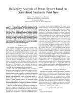
If the algorithm is stable the global error tends to zero even though the local
error may attain significant values.
Illustration of the errors discussed is shown in Fig.1.2. The plots presented have
been calculated for: y0 = 10; λ = 2; T = 0.987 [76].
a)

b)
ΔG

ΔL
3

10

3

2

1

3

5

1

1

0

0

–5 2

–1
–2 –4
10

2
10–3

10–2

10–1

T, s

100

–10
0

4

8

12

16

k

20

Fig. 1.2. Local ΔL and global ΔG error values for the algorithms considered: 1 – trapezoidal
approx.; 2 – Euler’s ‘step forward’ ; 3 – Euler’s ‘step backward’

1.3.

Numerical models of network elements

1.3.1. Resistance
As the resistive elements do not have the energy storing capacity the discrete relation
between current and voltage drop across resistance R can be obtained directly from the
continuous relation and:

i (k ) =

1
u (k ) = Gu (k )
R

(1.45)

1.3.2. Inductance
The energy stored in magnetic field produced by current has the impact on voltage

across the element so its continuous model is described by the equation:

di (t ) 1
= u (t )
dt
L

(1.46)


1.3. Numerical models of network elements

15

Using the transformation (1.6) or (1.9) the Euler’s implicit discrete model of the
element is obtained:

i (k ) = i (k − 1) +

T
u (k ) = i (k − 1) + Gu (k ),
L

G=

T
L

(1.47)

Note that T/L has the conductance unit.
For the trapezoidal transformation (1.7) or eqn.(1.10) the discrete model takes the
form:

i (k ) = i (k − 1) +

T
[u (k − 1) + u (k )]
2L

(1.48)

or

i ( k ) = Gu ( k ) + i ( k − 1) + Gu ( k − 1),

G=

T
2L

(1.49)

The eqn. (1.49) can be rearranged in the following way:

i(k ) = Gu(k ) + i(k − 1) + Gu(k − 1)

(1.50)

i (k ) = Gu(k ) + j (k − 1)

(1.51)

j (k − 1) = i(k − 1) + Gu (k − 1)

(1.52)

or

where

The calculations in step k employ the values calculated in step k–1 which are
constant and can be considered as the constant current sources j(k–1). Thus the
inductance can be represented by equivalent numerical model corresponding to (1.52)
which is shown in Fig.1.3.

a)
i(t)

b)
L

u(k)

i(k)
G

j(k-1)

u(t)

Fig. 1.3. Discrete model of inductance; a) symbol; b) numerical model


16

1. DISCRETE MODELS OF LINEAR ELECTRICAL NETWORK

1.3.3. Capacitance
This element also reveals the energy storing capacity in form of electric charge and the
relation between voltage and current in the element is given by the formula:

du (t ) 1
= i (t )
dt
C

(1.53)

Using the same transformations as for the inductance the discrete models of
capacitance can be derived:

u (k ) = u (k − 1) +

T
i (k )
C

(1.54)

Introducing the conductance notation (1.54) takes the form:

i (k ) = Gu (k ) − Gu ( k − 1),

G=

C
T

(1.55)

and

i ( k ) = Gu ( k ) + j ( k − 1),

j ( k − 1) = −Gu ( k − 1)

(1.56)

Using the trapezoidal integration method the discrete model of capacitance takes
the similar form:

u (k ) = u (k − 1) +

T
(i(k − 1) + i(k ))
2C

(1.57)

The companion discrete model for capacitance can be derived as:

i ( k ) = Gu ( k ) + j ( k − 1)

(1.58)

j ( k − 1) = −i ( k − 1) + Gu ( k − 1), G =

2C
T

(1.59)

The respective representation is shown in Fig.1.4:
a)
i(t)

C

b)

i(k)
u(k)

G

j(k-1)

u(t)

Fig. 1.4. Discrete model of capacitance; a) symbol; b) numerical model

1.3. Numerical models of network elements

17

In the very similar way the parameters of circuit representations for any integration
method used can be derived. In Table 1.1 the example of those parameters for three
selected methods are shown.
Table 1.1. Companion circuit parameters for selected numerical integration methods.
Integration method
Euler’s implicit
method
Trapezoidal
approximation

Model of inductance L
j ( k − 1) = i (k − 1) ,

Model of capacitance C
j (k − 1) = −Gu (k − 1) , G = C

T
G=
L

T

j ( k − 1) = i ( k − 1) + Gu ( k − 1) , G = T

2L

j (k − 1) =
nd

Gear’s 2 order

1
(4i(k − 1) − i (k − 2) ) ,
3
G=

2T
3L

j (k − 1) = −(i (k − 1) + Gu (k − 1) ) ,

G=

2C
T

1
⎛
⎞
j ( k − 1) = − G ⎜ 2 u ( k − 1 ) + u ( k − 2 ) ⎟
3
⎝
⎠
G=

3C
2T

Basic numerical algorithm: i ( k ) = Gu (k ) + j (k − 1)

1.3.4. Complex RLC branches
The equivalent discrete model of in series connected RLC branch can be obtained by
series connection of basic models of each particular element in the branch as it is
shown in Fig.1.5b.
b)

a)
i(t)
uR(t)

R

i(k)
GR

uR(k)

c)
i(k)
u(t)

uL(t)

L

uL(k)

GL

jL(k-1)

uC(t)

C

uC(k)

GC

jC(k-1)

u(k)

G

j(k-1)

Fig. 1.5. Discrete model of RLC branch; a) the continuous model; b) discrete models
of particular elements; c) the equivalent discrete model of the branch.


18

1. DISCRETE MODELS OF LINEAR ELECTRICAL NETWORK

To derive the equivalent discrete model (Fig. 1.5c) of the overall circuit consider
the basic equation for voltage across the branch (Fig. 1.5b):

u(k ) = uR (k ) + uL (k ) + uC (k )

(1.60)

in which the particular terms can be expressed by their basic models:

u R (k) =

1
i(k),
GR

u L (k ) =

1
(i(k) − j L (k −1)), uC (k) = 1 (i(k) − jC (k −1)).
GL
GC

(1.61)

After substitution and appropriate rearrangement of (1.60) the equivalent model
equation is obtained:

i(k) = Gu(k) + j(k −1)

(1.62)

in which, for trapezoidal approximation:
G=

GR GL GC
2CT
=
GR GL + GR GC + GL GC 4 LC + 2 RCT + T 2

j (k − 1) =

GR GC j L (k − 1) + GR GL jC (k − 1) G
G
=
j L (k − 1) +
jC (k − 1) ,
GR GL + GR GC + GL GC
GL
GC

1
, GL = T , GC = 2C .
R
2L
T
If capacitance C is not present in a branch then C→∞ must be put into the above
equations. For missing R or L, R = 0 or L = 0 must be used, respectively. For example,
in case of the R L branch the respective relations are:

and GR =

G=

T
2 L + RT

j (k − 1) =

2L
1 − RGL
jL (k − 1) =
i(k − 1) + Gu(k − 1)
2L + RT
1 + RGL

(1.63)

1.3.5. Controlled sources
Controlled sources are used very often in electronic and electric network models.
Generally there are four basic types of such sources (Fig.1.6) [18, 70]:
ƒ Voltage controlled current sources j = ku x controlled by voltage u x applied to
ƒ

control terminals.
Current controlled current sources j = ki x controlled by current i x injected

ƒ

into control terminals.

Voltage controlled voltage sources u = ku x .


1.3. Numerical models of network elements

ƒ

19

Current controlled voltage sources u = ki x .
a)
ux

ix

b)

j=kux

ix

j=kix

c)

d)
u=kix

ux

u=kux

Fig. 1.6. Diagrams of controlled sources; a) voltage controlled current source;
b) current controlled current source; c) current controlled voltage source;
d) voltage controlled voltage network.

Models of controlled sources are very simple; however, their implementation in
simulation programs may sometimes be cumbersome.
1.3.6. Frequency properties of discrete models
The frequency properties of discrete models are uniquely determined by the method
used for approximation of derivatives that appear in the continuous model of a given
element. Comparison of the continuous and the discrete models frequency properties
provides very useful information on how to select the calculation period T in order to
obtain the accurate enough transient component waveform of specified frequency fmax
which is present in the frequency spectrum of continuous transient voltages or
currents.
As an example let’s consider the discrete model of inductance obtained by use of
trapezoidal approximation. Using the already known relations (1.46, 1.13) we get:

1
2( z − 1)
i( z ) = u ( z )
T ( z + 1)
L
i( z ) =

T z +1
u( z)
2L z − 1

(1.64)
(1.65)

Now using (1.4) and remembering that in frequency domain s=jω :

i ( jω ) =

T e jωT + 1
u ( jω )
2 L e jωT − 1

(1.66)


20

1. DISCRETE MODELS OF LINEAR ELECTRICAL NETWORK

Applying rudimentary trigonometry knowledge the magnitude of the equation
(1.66) can be written in the following form:
i ( jω ) =

T
2
L tan

ωT

(1.67)

u ( jω )

2

Introducing the complex discrete admittances Yd(jω) and the continuous Yc(jω) we get:

T
Tω
Tω
i ( jω )
2
2
2 Y ( jω )
Yd ( jω ) =
=
=
=
c
u ( jω ) L tan ωT Lω tan ωT tan ωT
2
2
2

(1.68)

where Yc(jω) = 1/jLω is the admittance of the continuous model of inductance.
Thus, the ratio of the discrete admittance to the continuous one is given by:

Tω
Yd ( jω )

2
=
Yc ( jω ) tan ωT
2

(1.69)

and changes with frequency as it is shown in Fig. 1.7.
Yd
Y
0.9
0.8
0.7
0.6
0.5
0.4
0.3
0.2
0.1
0

0

0.1

0.2

0.3

0.4

0.5

ωT
2π

Fig. 1.7. Frequency response of discrete inductance model.


1.3. Numerical models of network elements

21

From eqn. (1.69) and from Fig. 1.7 one can notice that Yd(jω) reaches zero if
ωT
tan
→ ∞ This limit is reached when:
2

ωT
2

=

π
2

or

T=

1
π
π
=
=
ω 2πf 2 f

(1.70)

So if fmax is the frequency of the highest harmonic to be observed in current or
voltage signals then the calculation step T should be small enough according to
following condition:
T <<

1
2 f max

Practically, if required number of data samples within the period Tmax =

(1.71)

1
f max

is N

then (1.71) implies:

T ≤

1
Nf max

(1.72)

in which N must not be less than 2 (usually N > 20).
1.3.7. Distributed parameters model (long line model)

Distinction between lumped and distributed models of electric elements is made on the
basis of mutual relation between three basic parameters of the environment in which
the electromagnetic wave is propagated. These parameters are:
ƒ specific electric conductivity γ
ƒ relative magnetic permeability μ
ƒ relative electric permittivity ε
In case of lumped elements it is assumed that only one of the above listed
parameters is dominant and the remaining ones can be neglected. Thus particular
elements are deemed as lumped under following conditions:
ƒ μ = ε = 0 – lumped resistance
ƒ γ = ε = 0 – lumped inductance
ƒ γ = μ = 0 – lumped capacitance.
Additionally in case of lumped parameters model of an electric network the
electromagnetic field must be quasi-stationary; it means that in each point of the
network the electromagnetic field is practically the same or the differences are
negligibly small. In this respect the length of the electric conductor l is considered as


22

1. DISCRETE MODELS OF LINEAR ELECTRICAL NETWORK

the distinctive parameter. As the boundary value the length lgr equal to ¼ of the
electromagnetic wavelength propagated is assumed.
Thus, if the frequency of the propagated wave is f, than the lgr can be estimated as:
l gr =

λ
4

=

c
,
4f

(1.73)

c
is the wavelength.
f
then the length of the line can be neglected and can be modelled as the

where c is the velocity of light and λ =
If l << l gr

lumped parameter element. Otherwise ( l ≈ l gr ) the line should be considered as the
long one.
For example, if the transient harmonics of frequency f = 1000 Hz (the 20th
harmonic) may appear in the line during faults then l gr = c /( 4 f ) = 3 ⋅10 5 /(4 ⋅1000) =
75 km. The lightning stroke may induce much higher harmonics in the line so in such

case even a few kilometres long line should be represented by distributed parameters
model.
To derive the continuous model of the long line the equivalent Δx long segment of
the line shown in Fig.1.8 can be used. As Δx is assumed to be sufficiently short the
circuit parameters can be considered as the lumped ones.

i(x,t) R'Δx

L'Δx

G'Δx

u(x,t)

i(x+Δx,t)

C'Δx

u(x+Δx,t)
x+Δx

x

Fig.1.8. Elementary segment of a long line

The basic equations that describe the elementary line segment in Fig.1.8 are:

∂i ( x, t )
+ u ( x + Δx, t ),
∂t

∂u ( x + Δx, t )
i ( x, t ) = G ' Δx ⋅ u ( x + Δx, t ) + C ' Δx
+ i ( x + Δx, t ),
∂t

u ( x, t ) = R ' Δx ⋅ i ( x, t ) + L' Δx

(1.74)

where: R ' , L' , G ' , C ' denote ‘unit/ length’ values of resistance, inductance and
capacitance of the line, respectively.


1.3. Numerical models of network elements

23

Dividing both equations by Δx and taking the limes ( Δx → 0 ) the following
relations are obtained:

∂u ( x, t )
∂i ( x, t )
= R ' i ( x, t ) + L '
,
∂x
∂t
∂i ( x, t )
∂u ( x, t )
−
= G ' u ( x, t ) + C '

.
∂x
∂t
−

(1.75)

If the line is homogenous then (1.75) can be separated with respect to current and
voltage (for simplicity: u = u ( x, t ) , i = i ( x, t ) ):
−

∂u 2
∂u
∂i 2
=
−
R
G
u
−
R
C
+
L
'
'
'
'
'
∂t

∂x∂t
∂x 2

(1.76)

and
∂u 2
∂u
∂u 2
(
)
=
+
+
R
G
u
R
C
G
L
+
'
'
'
'
'
'
L
'

C
'
∂t
∂x 2
∂t 2

(1.77)

Applying the same simplifying procedure to the second equation in (1.75) the
respective relation for current can be obtained:
∂i 2
∂i
∂i 2
(
)
=
R
'
G
'
i
+
R
'
C
'
+
G
'
L

'
+
L
'
C
'
∂t
∂x 2
∂t 2

(1.78)

Both (1.75) and (1.76) are the second order hyperbolic partial differential equations
known as telegraph equations [80].
a)

Lossless (non-dissipating) long line

This case is obtained under assumption that R ' = 0 and G '= 0 and the resulting
simplification of (3.4) and (3.5) is:

∂u 2 1 ∂u 2
−
= 0,
∂x 2 v 2 ∂t 2
∂i 2
1 ∂i 2
−
= 0.
∂x 2 v 2 ∂t 2

(1.79)

in which:
v=

1
L' C '

(1.80)


24

1. DISCRETE MODELS OF LINEAR ELECTRICAL NETWORK

The general solution of (3.6) has been found by d’Alembert [24, 28]. For the
following boundary conditions:
u ( x, t ) x=0 = ϕ (t ) ,

∂u ( x, t )
∂x

= ψ (t )
x =0

the solution of (1.79) takes the form:
u ( x, t ) =

1

(ϕ (t + x / v) + ϕ (t − x / v) ) + v
2
2

∫

t + x/v

t -x/v

ψ (α )dα

(1.81)

The loci of points (t − x / v) = const and (t + x / v) = const known as propagation
characteristics of (1.81) [6, 39] show the propagation mechanism of ϕ ( x, t ) waves in a
long line.
t

t-x/v=const

t+x/v=const

tp

xp

x1

x2

x

Fig. 1.9. Propagation characteristics of a lossless long line

The boundary conditions expressed in terms of voltage u1 (t ) and current i1 (t ) at
the beginning of the lossless ( R' = 0 ) line (1.75) yields:
ϕ (t ) = u (0, t ) = u1 (t ) , ψ (t ) =

di (t )
∂u (0, t )
∂i (0, t )
= − L'
= − L' 1
∂x
∂t
dt

and the solution (1.81) takes the form:

u ( x, t ) =

1
(u1 (t + x / v) + u1 (t − x / v) ) − 1 Z f
2
2

∫

t + x/v

t -x/v

dii (t )

L'
is the wave (surge) impedance of the line.
C'
For x = l (end of the line) solution of (1.82) is given by the equation:

where Z f =

(1.82)


1.3. Numerical models of network elements

25

1
(u1 (t + τ ) + u1 (t − τ ) ) − 1 Z f (i1 (t + τ ) − i1 (t − τ ) )
2
2

u 2 (t ) =

(1.83)

where: τ = l / v is the line propagation time.
Similarly, the wave equation for current can be obtained and:

i2 (t ) = −

1
(i1 (t + τ ) + i1 (t − τ ) ) + 1 (u1 (t + τ ) − u1 (t − τ ) )
2
2Z f

(1.84)

Note that it was assumed that the current at the end of the line flows in reverse
direction with respect to the current at the line beginning (see Fig.1.8) and that is why
it bears the opposite sign.
Subtracting (1.83) from (1.84) the model of the long lossless line is obtained:
i2 (t ) = G f u 2 (t ) − G f u1 (t − τ ) − i1 (t − τ )
where: G f =

(1.85)

1
.
Zf
1 i1

i2

2

u2

u1

x

Fig.1.10. Assignment of variables in the lossless line

When the boundary conditions are assigned to the beginning and to the end of the
line, the solution concerns these two points only. The propagation characteristics also
comprise of 2 points: x1 = 0 and x2 = l . This simple model is called the Bergeron’s
model [24, 49].
The continuous model (1.85) of the lossless line can easily be converted into the
discrete one. Assuming that wave propagation time is mT = τ then:

m=

τ
T

=

l
vT

(1.86)

and
i2 (k ) = G f u 2 (k ) − G f u1 (k − m) − ii ( k − m)

(1.87)