Tin học trong công nghệ hóa học và thực phẩm English
Bạn đang xem bản rút gọn của tài liệu. Xem và tải ngay bản đầy đủ của tài liệu tại đây (3.04 MB, 243 trang )
PRO/II Unit Operations
Reference Manual
The software described in this manual is furnished under a license
agreement and may be used only in accordance with the terms of that
agreement.
Information in this document is subject to change without notice.
Simulation Sciences Inc. assumes no liability for any damage to any
hardware or software component or any loss of data that may occur as
a result of the use of the information contained in this manual.
Copyright Notice
Copyright © 1994 Simulation Sciences Inc. All Rights Reserved. No
part of this publication may be copied and/or distributed without the
express written permission of Simulation Sciences Inc., 601 S. Valencia
Avenue, Brea, CA 92621, USA.
Trademarks
PRO/II is a registered mark of Simulation Sciences Inc.
PROVISION is a trademark of Simulation Sciences Inc.
SIMSCI is a service mark of Simulation Sciences Inc.
Printed in the United States of America.
Credits
Contributors:
Miguel Bagajewicz, Ph.D.
Ron Bondy
Bruce Cathcart
Althea Champagnie, Ph.D.
Joe Kovach, Ph.D.
Grace Leung
Raj Parikh, Ph.D.
Claudia Schmid, Ph.D.
Vasant Shah, Ph.D.
Richard Yu, Ph.D.
Table of Contents
List of Tables
TOC-6
List of Figures
TOC-7
Introduction
INT-1
General Information
What is in This Manual?
Who Should Use This Manual?
Finding What You Need
Flash Calculations
Basic Principles
MESH Equations
ii-1
ii-1
ii-1
ii-1
II-3
II-4
II-4
Two-phase Isothermal Flash Calculations
Flash Tolerances
II-5
II-8
Bubble Point Flash Calculations
II-8
Dew Point Flash Calculations
Two-phase Adiabatic Flash Calculations
II-9
II-9
Water Decant
II-9
Three-phase Flash Calculations
Equilibrium Unit Operations
Flash Drum
Valve
II-11
II-12
II-12
II-13
Mixer
II-13
Splitter
II-14
Isentropic Calculations
II-17
Compressor
General Information
Basic Calculations
II-19
ASME Method
GPSA Method
II-21
II-23
General Information
Basic Calculations
II-25
II-25
II-25
Expander
Pressure Calculations
Pipes
PRO/II Unit Operations Reference Manual
II-18
II-18
II-31
General Information
II-32
II-32
Basic Calculations
Pressure Drop Correlations
II-32
II-34
Table of Contents
TOC-1
Pumps
General Information
Basic Calculations
II-41
II-41
II-41
Distillation and Liquid-Liquid Extraction Columns
II-45
Rigorous Distillation Algorithms
General Information
II-46
II-46
General Column Model
Mathematical Models
II-47
II-49
Inside Out Algorithm
II-50
Chemdist Algorithm
Reactive Distillation Algorithm
II-56
II-60
Initial Estimates
ELDIST Algorithm
Basic Algorithm
II-65
II-69
II-69
Column Hydraulics
General Information
II-73
II-73
Tray Rating and Sizing
Random Packed Columns
II-73
II-76
Structured Packed Columns
II-80
Shortcut Distillation
General Information
Fenske Method
II-85
Underwood Method
Kirkbride Method
II-86
II-89
Gilliland Correlation
II-89
Distillation Models
Troubleshooting
II-90
II-96
Liquid-Liquid Extractor
General Information
Basic Algorithm
Heat Exchangers
TOC-2
Table of Contents
II-85
II-85
II-100
II-100
II-100
II-105
Simple Heat Exchangers
General Information
Calculation Methods
II-106
II-106
II-106
Zones Analysis
General Information
Calculation Methods
II-109
II-109
II-109
Example
II-110
Rigorous Heat Exchanger
General Information
II-112
II-112
Heat Transfer Correlations
Pressure Drop Correlations
II-114
II-116
Fouling Factors
II-120
LNG Heat Exchanger
General Information
II-122
II-122
Calculation Methods
Zones Analysis
II-122
II-124
May 1994
Reactors
II-127
Reactor Heat Balances
Heat of Reaction
II-128
II-129
Conversion Reactor
Shift Reactor Model
II-130
II-131
Methanation Reactor Model
Equilibrium Reactor
Shift Reactor Model
Methanation Reactor Model
Calculation Procedure for Equilibrium
II-131
II-132
II-134
II-134
II-135
Gibbs Reactor
General Information
Mathematics of Free Energy Minimization
II-136
II-136
II-136
Continuous Stirred Tank Reactor (CSTR)
Design Principles
II-141
II-141
Multiple Steady States
II-143
Boiling Pot Model
CSTR Operation Modes
II-144
II-144
Plug Flow Reactor (PFR)
Design Principles
PFR Operation Modes
Solids Handling Unit Operations
Dryer
II-145
II-145
II-147
II-151
General Information
Calculation Methods
II-152
II-152
II-152
Rotary Drum Filter
General Information
Calculation Methods
II-153
II-153
II-153
Filtering Centrifuge
General Information
II-157
II-157
Calculation Methods
II-157
Countercurrent Decanter
General Information
II-161
II-161
Calculation Methods
II-161
Calculation Scheme
General Information
Development of the Dissolver Model
II-163
II-165
II-165
II-165
Mass Transfer Coefficient Correlations
II-167
Particle Size Distribution
Material and Heat Balances and Phase Equilibria
II-168
II-168
Solution Procedure
II-170
Crystallizer
General Information
II-171
II-171
Dissolver
PRO/II Unit Operations Reference Manual
Crystallization Kinetics and Population
Balance Equations
II-172
Material and Heat Balances and Phase Equilibria
II-175
Solution Procedure
II-176
Table of Contents
TOC-3
Melter/Freezer
General Information
Calculation Methods
Stream Calculator
II-183
Feed Blending Considerations
II-183
Stream Splitting Considerations
Stream Synthesis Considerations
II-184
II-185
II-189
Phase Envelope
General Information
II-190
II-190
Calculation Methods
Heating / Cooling Curves
General Information
II-190
II-192
II-192
Calculation Options
Critical Point and Retrograde Region Calculations
II-192
II-193
VLE, VLLE, and Decant Considerations
II-194
Water and Dry Basis Properties
GAMMA and KPRINT Options
II-194
II-194
Availability of Results
Binary VLE/VLLE Data
General Information
II-195
II-198
II-198
Input Considerations
Output Considerations
II-198
II-199
General Information
II-200
II-200
Theory
II-200
General Information
II-206
II-206
Interpreting Exergy Reports
II-206
Hydrates
Exergy
Flowsheet Solution Algorithms
Sequential Modular Solution Technique
General Information
Methodology
Process Unit Grouping
II-211
II-212
II-212
II-212
II-213
Calculation Sequence and Convergence
General Information
II-215
II-215
Tearing Algorithms
Convergence Criteria
II-215
II-217
Acceleration Techniques
General Information
Wegstein Acceleration
Broyden Acceleration
Table of Contents
II-183
General Information
Utilities
TOC-4
II-178
II-178
II-178
II-218
II-218
II-218
II-219
Flowsheet Control
General Information
II-221
II-221
Feedback Controller
General Information
II-222
II-222
May 1994
Multivariable Feedback Controller
General Information
Flowsheet Optimization
General Information
Solution Algorithm
Depressuring
Index
PRO/II Unit Operations Reference Manual
II-226
II-226
II-229
II-229
II-234
II-241
General Information
Theory
II-241
II-241
Calculating the Vessel Volume
II-242
Valve Rate Equations
Heat Input Equations
II-243
II-245
1-1
Table of Contents
TOC-5
List of Tables
TOC-6
2.1.1-1
Flash Tolerances . . . . . . . . . . . . . . . . . . . . . . . . . II-8
2.1.1-1
VLLE Predefined Systems and K-value Generators . . . . . . . II-11
2.1.2-1
Constraints in Flash Unit Operation . . . . . . . . . . . . . . . II-12
2.2.1-1
Thermodynamic Generators for Entropy . . . . . . . . . . . . II-18
2.3.1-1
Thermodynamic Generators for Viscosity and Surface Tension
2.4.1-1
Features Overview for Each Algorithm . . . . . . . . . . . . . II-48
2.4.1-2
Default and Available IEG Models . . . . . . . . . . . . . . . . II-67
2.4.3-1
Thermodynamic Generators for Viscosity . . . . . . . . . . . II-73
2.4.3-2
System Factors for Foaming Applications . . . . . . . . . . . II-74
2.4.3-3
Random Packing Types, Sizes, and Built-in Packing Factors . . II-77
2.4.3-4
Types of Sulzer Packings Available in PRO/II . . . . . . . . . . II-81
2.4.4-1
Typical Values of FINDEX . . . . . . . . . . . . . . . . . . . . II-95
2.4.4-2
Effect of Cut Ranges on Crude Unit Yields Incremental
Yields from Base . . . . . . . . . . . . . . . . . . . . . . . . II-98
2.7.3-1
Types of Filtering Centrifuges Available in PRO/II . . . . . . . . II-157
2.9.2-1
GAMMA and KPRINT Report Information . . . . . . . . . . . . II-195
2.9.2-1
Sample HCURVE .ASC File . . . . . . . . . . . . . . . . . . . II-196
2.9.2-3
Data For an HCURVE Point . . . . . . . . . . . . . . . . . . . II-196
2.9.4-1
Properties of Hydrate Types I and II . . . . . . . . . . . . . . II-200
2.9.4-2
Hydrate-forming Gases . . . . . . . . . . . . . . . . . . . II-201
2.9.5-1
Availability Functions . . . . . . . . . . . . . . . . . . . . . . II-207
2.10.2-1
Possible Calculation Sequences . . . . . . . . . . . . . . . . . II-216
2.10.3-1
Significance of Values of the Acceleration Factor, q . . . . . . II-218
2.10.4-1
General Flowsheet Tolerances . . . . . . . . . . . . . . . . . . II-221
2.10.5-1
Diagnostic Printout . . . . . . . . . . . . . . . . . . . . . . . II-236
2.11-1
Value of Constant A . . . . . . . . . . . . . . . . . . . . . . . II-245
2.11-2
Value of Constants C , C . . . . . . . . . . . . . . . . . . . . II-246
Table of Contents
II-32
May 1994
List of Figures
2.1.1-1
Three-phase Equilibrium Flash . . . . . . . . . . . . . . . . . II-4
2.1.1-2
Flowchart for Two-phase T, P Flash Algorithm . . . . . . . . . II-6
2.1.2-1
Valve Unit . . . . . . . . . . . . . . . . . . . . . . . . . . . . II-13
2.1.2-2
Mixer Unit . . . . . . . . . . . . . . . . . . . . . . . . . . . . II-13
2.1.2-3
Splitter Unit . . . . . . . . . . . . . . . . . . . . . . . . . . . II-14
2.2.1-1
Polytropic Compression Curve . . . . . . . . . . . . . . . . . II-19
2.2.1-2
Typical Mollier Chart for Compression . . . . . . . . . . . . . II-20
2.2.2-1
Typical Mollier Chart for Expansion . . . . . . . . . . . . . . . II-25
2.3.1-1
Various Two-phase Flow Regimes . . . . . . . . . . . . . . . II-36
2.4.1-1
Schematic of Complex Distillation Column . . . . . . . . . . . II-47
2.4.1-2
Schematic of a Simple Stage for I/O . . . . . . . . . . . . . . II-51
2.4.1-3
Schematic of a Simple Stage for Chemdist . . . . . . . . . . . II-56
2.4.1-4
Reactive Distillation Equilibrium Stage . . . . . . . . . . . . . II-61
2.4.2-1
ELDIST Algorithm Schematic . . . . . . . . . . . . . . . . . . II-69
2.4.3-1
Pressure Drop Model . . . . . . . . . . . . . . . . . . . . . . II-83
2.4.4-1
Algorithm to Determine Rmin . . . . . . . . . . . . . . . . . . II-88
2.4.4-2
Shortcut Distillation Column Condenser Types . . . . . . . . . II-89
2.4.4-3
Shortcut Distillation Column Models . . . . . . . . . . . . . . II-90
2.4.4-4
Shortcut Column Specification . . . . . . . . . . . . . . . . . II-92
2.4.4-5
Heavy Ends Column . . . . . . . . . . . . . . . . . . . . . . . II-94
2.4.4-6
Crude- Preflash System . . . . . . . . . . . . . . . . . . . . . II-94
2.4.5-1
Schematic of a Simple Stage for LLEX . . . . . . . . . . . . . II-100
2.5.1-1
Heat Exchanger Temperature Profiles . . . . . . . . . . . . . . II-107
2.5.2-1
Zones Analysis for Heat Exchangers . . . . . . . . . . . . . . II-110
2.5.3-1
TEMA Heat Exchanger Types . . . . . . . . . . . . . . . . . . II-113
2.5.4-2
LNG Exchanger Solution Algorithm . . . . . . . . . . . . . . . II-123
2.6.1-1
Reaction Path for Known Outlet Temperature and Pressure . . II-128
2.6.5-1
Continuous Stirred Tank Reactor . . . . . . . . . . . . . . . . II-141
2.6.5-2
Thermal Behavior of CSTR . . . . . . . . . . . . . . . . . . . II-143
2.6.6-1
Plug Flow Reactor . . . . . . . . . . . . . . . . . . . . . . . . II-145
2.7.4-1
Countercurrent Decanter Stage . . . . . . . . . . . . . . . . . II-161
2.7.5-1
Continuous Stirred Tank Dissolver . . . . . . . . . . . . . . . II-166
2.7.6-1
Crystallizer . . . . . . . . . . . . . . . . . . . . . . . . . . . . II-172
2.7.6-2
Crystal Particle Size Distribution . . . . . . . . . . . . . . . . II-173
PRO/II Unit Operations Reference Manual
Table of Contents
TOC-7
TOC-8
2.7.6-3
MSMPR Crystallizer Algorithm . . . . . . . . . . . . . . . . . II-177
2.7.7-1
Calculation Scheme for Melter/Freezer . . . . . . . . . . . . . II-179
2.9.1-1
Phase Envelope . . . . . . . . . . . . . . . . . . . . . . . . . II-190
2.9.2-1
Phenomenon of Retrograde Condensation . . . . . . . . . . . II-193
2.9.4-1
Unit Cell of Hydrate Types I and II . . . . . . . . . . . . . . . . II-201
2.9.4-2
Method Used to Determine Hydrate-forming Conditions . . . . II-204
2.10.1-1
Flowsheet with Recycle . . . . . . . . . . . . . . . . . . . . . II-212
2.10.1-2
Column with Sidestrippers . . . . . . . . . . . . . . . . . . . II-214
2.10.2-1
Flowsheet with Recycle . . . . . . . . . . . . . . . . . . . . . II-216
2.10.4.1-1
Feedback Controller Example . . . . . . . . . . . . . . . . . . II-222
2.10.4.1-2
Functional RelationshipBetween Control Variable and
Specification . . . . . . . . . . . . . . . . . . . . . . . . . . . II-223
2.10.4.1-3
Feedback Controller in Recycle Loop . . . . . . . . . . . . . . II-224
2.10.4.2-1
Multivariable Controller Example . . . . . . . . . . . . . . . . II-226
2.10.4.2-2
MVC SolutionTechnique . . . . . . . . . . . . . . . . . . . . . II-227
2.10.5-1
Optimization of Feed Tray Location . . . . . . . . . . . . . . . II-230
2.10.5-2
Choice of Optimization Variables . . . . . . . . . . . . . . . . II-232
Table of Contents
May 1994
Introduction
General
Information
What is in
This Manual?
The PRO/II Unit Operations Reference Manual provides details on the basic
equations and calculation techniques used in the PRO/II simulation program. It
is intended as a complement to the PRO/II Keyword Input Manual, providing a
reference source for the background behind the various PRO/II calculation
methods.
This manual contains the correlations and methods used for the various unit
operations, such as the Inside/Out and Chemdist column solution algorithms.
For each method described, the basic equations are presented, and appropriate references provided for details on their derivation. General application
guidelines are provided, and, for many of the methods, hints to aid solution
are supplied.
Who Should Use
This Manual?
For novice, average, and expert users of PRO/II, this manual provides a good
overview of the calculation modules used to simulate a single unit operation
or a complete chemical process or plant. Expert users can find additional
details on the theory presented in the numerous references cited for each
topic. For the novice to average user, general references are also provided on
the topics discussed, e.g., to standard textbooks.
Specific details concerning the coding of the keywords required for the
PRO/II input file can be found in the PRO/II Keyword Input Manual.
Detailed sample problems are provided in the PRO/II Application Briefs
Manual and in the PRO/II Casebooks.
Finding What
you Need
A Table of Contents and an Index are provided for this manual. Crossreferences are provided to the appropriate section(s) of the PRO/II Keyword
Input Manual for help in writing the input files.
PRO/II Unit Operations Reference Manual
Introduction
Int-1
Symbols Used in This Manual
Symbol
Meaning
Indicates a PRO/II input coding note. The number beside the
symbol indicates the section in the PRO/II Keyword Input
Manual to refer to for more information on coding the
input file.
Indicates an important note.
Indicates a list of references.
Int-2
Introduction
May 1994
This page intentionally left blank.
II-2
May 1994
Section 2.1
2.1
Flash Calculations
Flash Calculations
PRO/II contains calculations for equilibrium flash operations such as flash
drums, mixers, splitters, and valves. Flash calculations are also used to determine
the thermodynamic state of each feed stream for any unit operation. For a flash calculation on any stream, there are a total of NC + 3 degrees of freedom, where NC is the
number of components in the stream. If the stream composition and rate are fixed,
then there are 2 degrees of freedom that may be fixed. These may, for example, be
the temperature and pressure (an isothermal flash). In addition, for all unit operations, PRO/II also performs a flash calculation on the product streams at the outlet
conditions. The difference in the enthalpy of the feed and product streams constitutes
the net duty of that unit operation.
PRO/II Unit Operations Reference Manual
II-3
Flash Calculations
2.1.1
Section 2.1
Basic Principles
Figure 2.1.1-1 shows a three-phase equilibrium flash.
Figure 2.1.1-1:
Three-phase
Equilibrium Flash
MESH
Equations
The Mass balance, Equilibrium, Summation, and Heat balance (or MESH)
equations which may be written for a three-phase flash are given by:
Total Mass Balance:
F = V + L1 + L2
(1)
Component Mass Balance:
Fzi = Vyi + L1 + L2
(2)
Equilibrium:
yi = K1i x1i
(3)
yi = K2i x2i
(4)
x1i =
K2i
x
K1i 2i
(5)
Summations:
∑
i
∑
i
II-4
Basic Principles
yi − ∑ x1i = 0
(6)
i
yi − ∑ x2i = 0
(7)
i
May 1994
Section 2.1
Flash Calculations
Heat Balance:
FHf + Q = VHv + L1H1l + L2H2l
Two-phase
Isothermal Flash
Calculations
(8)
For a two-phase flash, the second liquid phase does not exist, i.e., L2 = 0,
and L1 = L in equations (1) through (8) above. Substituting in equation (2)
for L from equation (1), we obtain the following expression for the liquid
mole fraction, xi:
xi =
(9)
zi
V
(Ki − 1) + 1
F
The corresponding vapor mole fraction is then given by:
yi = Kixi
(10)
The mole fractions, xi and yi sum to 1.0, i.e.:
∑
i
xi = ∑ yi = 1.0
(11)
i
However, the solution of equation (11) often gives rise to convergence difficulties for problems where the solution is reached iteratively. Rachford and Rice in
1952 suggested that the following form of equation (11) be used instead:
∑
i
yi − ∑ xi = ∑
i
i
(Ki − 1) zi
(Ki − 1)
V
+1
F
(12)
≤ TOL
Equation (12) is easily solved iteratively by a Newton-Raphson technique,
with V/F as the iteration variable.
Figure 2.1.1-2 shows the solution algorithm for a two-phase isothermal flash,
i.e., where both the system temperature and pressure are given. The following steps outline the solution algorithm.
1.
The initial guesses for component K-values are obtained from ideal
K-value methods. An initial value of V/F is assumed.
2.
Equations (9) and (10) are then solved to obtain xi’s and yi’s.
3.
After equation (12) is solved within the specified tolerance, the composition convergence criteria are checked, i.e., the changes in the vapor and
liquid mole fraction for each component from iteration to iteration are
calculated:
| (yi,ITER − yi,ITER−1) |
yi
PRO/II Unit Operations Reference Manual
≤ TOL
(13)
Basic Principles
II-5
Flash Calculations
Section 2.1
Figure 2.1.1-2:
Flowchart for
Two-phase T, P
Flash Algorithm
II-6
Basic Principles
May 1994
Section 2.1
Flash Calculations
Figure 2.1.1-2:, continued
Flowchart for
Two-phase T, P
Flash Algorithm
| (xi,ITER − xi,ITER−1) |
xi
(14)
≤ TOL
4.
If the compositions are still changing from one iteration to the next, a
damping factor is applied to the compositions in order to produce a stable
convergence path.
5.
Finally, the VLE convergence criterion is checked, i.e., the following condition must be met:
| ∑ y − ∑ x
i
|
− ∑ yi − ∑ xi
≤ TOL
ITER
ITER−1
i
(15)
If the VLE convergence criterion is not met, the vapor and liquid mole
fractions are damped, and the component K-values are re-calculated. Rigorous K-values are calculated using equation of state methods, generalized
correlations, or liquid activity coefficient methods.
6.
A check is made to see if the current iteration step, ITER, is greater than the
maximum number of iteration steps ITERmax. If ITER > ITERmax, the flash
has failed to reach a solution, and the calculations stop. If ITER < ITERmax,
the calculations continue.
7.
Steps 2 through 6 are repeated until the composition convergence criteria and
the VLE criterion are met. The flash is then considered solved.
8.
Finally, the heat balance equation (8) is solved for the flash duty, Q, once
V and L are known.
PRO/II Unit Operations Reference Manual
Basic Principles
II-7
Flash Calculations
Flash
Tolerances
Section 2.1
The flash equations are solved within strict tolerances. All these tolerances
are built into the PRO/II flash algorithm, and may not be input by the user.
Table 2.1.1-1 shows the values of the tolerances used in the algorithm for the
Rachford-Rice equation (12), the composition convergence equations (13)
and (14), and the VLE convergence equation (15).
Table 2.1.1-1: Flash Tolerances
Equation
Bubble Point
Flash Calculations
Tolerance
Rachford-Rice (12)
1.0e-05
Composition Convergence
(13-14)
1.0e-03
VLE Convergence (15)
1.0e-05
For bubble point flashes, the liquid phase component mole fractions, xi, still
equal the component feed mole fraction, zi. Moreover, the amount of vapor,
V, is equal to zero. Therefore, the relationship to be solved is:
∑i Kizi = ∑i yi = 1.0
(16)
The bubble point temperature or pressure is to be found by trial-and-error
Newton-Raphson calculations, provided one of them is specified.
The K-values between the liquid and vapor phase are calculated by the thermodynamic method selected by the user. Equation (16) can, however, be
highly non-linear as a function of temperature as K-values typically vary as
exp(1/T). For bubble point temperature calculations, where the pressure and
feed compositions has been given, and only the temperature is to be determined, equation (16) can be rewritten as:
ln∑ Ki zi = 0
i
(17)
Equation (17) is more linear in behavior than equation (16) as a function of
temperature, and so a solution can be achieved more readily.
Equation (16) behaves in a more linear fashion as a function of pressure as
the K-values vary as 1/P. For bubble point pressure calculations, where the
temperature and feed compositions have been given, the equation to be
solved can be written as:
∑
Kizi − 1 = 0
(18)
i
II-8
Basic Principles
May 1994
Section 2.1
Dew Point Flash
Calculations
Flash Calculations
A similar technique is used to solve a dew point flash. The amount of vapor,
V, is equal to 1.0. Simplification of the mass balance equations result in the
following relationship:
∑i zi / Ki = ∑ xi = 1.0
(19)
i
For dew point pressure calculations, equation (19) can be linearized by writing it as :
ln ∑
i
zi
=0
Ki
(20)
For dew point temperature calculations, equation (19) may be rewritten as:
∑
i
zi
−1=0
Ki
(21)
The dew point temperature or pressure is then found by trial-and-error Newton-Raphson calculations using equations (20) or (21).
Two-phase
Adiabatic Flash
Calculations
For a two-phase, adiabatic (Q=0) system, the heat balance equation (8) can
be rewritten as:
1−
Hv
Hf
V Hl
− 1 − ≤ TOL
F
Hf
(22)
An iterative Newton-Raphson technique is used to solve the Rachford-Rice
equation (12) simultaneously with equation (22) using V/F and temperature
as the iteration variables.
Water Decant
The water decant option in PRO/II is a special case of a three-phase flash. If this
option is chosen, and water is present in the system, a pure water phase is decanted
as the second liquid phase, and this phase is not considered in the equilibrium flash
computations. This option is available for a number of thermodynamic calculation
methods such as Soave-Redlich-Kwong or Peng-Robinson.
Note: The free-water decant option may only be used with the Soave-RedlichKwong, Peng-Robinson, Grayson-Streed, Grayson-Streed-Erbar, Chao-Seader,
Chao-Seader-Erbar, Improved Grayson-Streed, Braun K10, or Benedict-WebbRubin-Starling methods. Note that water decant is automatically activated
when any one of these methods is selected.
PRO/II Unit Operations Reference Manual
Basic Principles
II-9
Flash Calculations
Section 2.1
The water-decant flash method as implemented in PRO/II follows these steps:
20.6
1.
Water vapor is assumed to form an ideal mixture with the hydrocarbon vapor phase.
2.
Once either the system temperature, or pressure is specified, the initial
value of the iteration variable, V/F is selected and the water partial pressure is calculated using one of two methods.
3.
The pressure of the system, P, is calculated on a water-free basis, by
subtracting the water partial pressure.
4.
A pure water liquid phase is formed when the partial pressure of water
reaches its saturation pressure at that temperature.
5.
A two phase flash calculation is done to determine the hydrocarbon vapor
and liquid phase conditions.
6.
The amount of water dissolved in the hydrocarbon-rich liquid phase is
computed using one of a number of water solubility correlations.
7.
Steps 2 through 6 are repeated until the iteration variable is solved within
the specified tolerance.
PRO/II Note: For more information on using the free-water decant option, see
Section 20.6, Free-Water Decant Considerations, of the PRO/II Keyword Input
Manual.
References
II-10
Basic Principles
1.
Perry R. H., and Green, D.W., 1984, Chemical Engineering Handbook, 6th Ed.,
McGraw-Hill, N.Y.
2.
Rachford, H.H., Jr., and Rice, J.D., 1952, J. Petrol. Technol., 4 sec.1, 19,
sec. 2,3.
3.
Prausnitz, J.M., Anderson, T.A., Grens, E.A., Eckert, C.A., Hsieh, R., and
O’Connell, J.P., 1980, Computer Calculations for Multicomponent VaporLiquid and Liquid-Liquid Equilibria, Prentice-Hall, Englewood Cliffs, N.J.
May 1994
Section 2.1
Three-phase
Flash
Calculations
Flash Calculations
For three-phase flash calculations, with a basis of 1 moles/unit time of feed,
F, the MESH equations are simplified to yield the following two nonlinear
equations:
| f1(L1, L2) | = | ∑ai zi / di | ≤ tolerance
(23)
i
| f1(L1, L2) | = | ∑bi zi / di | ≤ tolerance
(24)
i
where:
ai = (1 − K1i)
(25)
bi = (1 − K2i) (K1i / K2i)
(26)
di = K1i + ai L1 + bi L2
(27)
Equations (23) through (27) are solved iteratively using a Newton-Raphson
technique to obtain L1 and L2. The solution algorithm developed by SimSci
is able to rigorously predict two liquid phases. This algorithm works well
even near the plait point, i.e., the point on the ternary phase diagram where a
single phase forms.
Table 2.1.1-1 shows the thermodynamic methods in PRO/II which are able to
handle VLLE calculations. For most methods, a single set of binary
interaction parameters is inadequate for handling both VLE and LLE equilibria. The PRO/II databanks contain separate sets of binary interaction parameters for VLE and LLE equilibria for many of the thermodynamic
methods available in PRO/II, including the NRTL and UNIQUAC liquid activity methods. For best results, the user should always ensure that separate
binary interaction parameters for VLE and LLE equilibria are provided for
the simulation.
Table 2.1.1-1:
VLLE Predefined Systems and K-value Generators
K-value Method
SRK1
SRKM
SRKKD
SRKH
SRKP
SRKS
PR1
PRM
PRH
PRP
UNIWAALS
IGS
GSE
CSE
HEXAMER
1
AMINE
NRTL
UNIQUAC
UNIFAC
UFT1
UFT2
UFT3
UNFV
VANLAAR
MARGULES
REGULAR
FLORY
SOUR
GPSWATER
LKP
System
SRK1
SRKM
SRKKD
SRKH
SRKP
SRKS
PR1
PRM
PRH
PRP
UNIWAALS
IGS
GSE
CSE
AMINE
HEXAMER
NRTL
UNIQUAC
UNIFAC
UFT1
UFT2
UFT3
UNFV
VANLAAR
MARGULES
REGULAR
FLORY
ALCOHOL
GLYCOL
SOUR
GPSWATER
LKP
VLLE available, but not recommended
PRO/II Unit Operations Reference Manual
Basic Principles
II-11
Flash Calculations
2.1.2
Section 2.1
Equilibrium Unit Operations
Flash
Drum
The flash drum unit can be operated under a number of different fixed conditions; isothermal (temperature and pressure specified), adiabatic (duty specified), dew point (saturated vapor), bubble point (saturated liquid), or isentropic
(constant entropy) conditions. The dew point may also be determined for the hydrocarbon phase or for the water phase. In addition, any general stream specification such as a component rate or a special stream property such as sulfur content
can be made at either a fixed temperature or pressure. For the flash drum unit,
there are two other degrees of freedom which may be set by imposing external
specifications. Table 2.1.2-1 shows the 2-specification combinations which may
be made for the flash unit operation.
Table 2.1.2-1:
Constraints in Flash Unit Operation
Flash Operation
Specification 1
ISOTHERMAL
TEMPERATURE
PRESSURE
DEW POINT
TEMPERATURE
PRESSURE
V=1.0
V=1.0
BUBBLE POINT
TEMPERATURE
PRESSURE
V=0.0
V=0.0
ADIABATIC
TEMPERATURE
PRESSURE
FIXED DUTY
FIXED DUTY
ISENTROPIC
TEMPERATURE
PRESSURE
FIXED ENTROPY
FIXED ENTROPY
TPSPEC
TEMPERATURE
GENERAL STREAM
SPECIFICATION
GENERAL STREAM
SPECIFICATION
PRESSURE
II-12
Specification 2
Equilibrium Unit Operations
May 1994
Section 2.1
Flash Calculations
Valve
Figure 2.1.2-1:
Valve Unit
The valve unit operates in a similar manner to an adiabatic flash. The outlet
pressure, or the pressure drop across the valve is specified, and the temperature of the outlet streams is computed for a total duty specification of 0. The
outlet product stream may be split into separate phases. Both VLE and VLLE
calculations are allowed for the valve unit. One or more feed streams are allowed for this unit operation.
Mixer
Figure 2.1.2-2:
Mixer Unit
The mixer unit is, like the valve unit operation, solved in a similar manner to
that of an adiabatic flash unit. In this unit, the temperature of the single outlet stream is computed for a specified outlet pressure and a duty specification
of zero. The number of feed streams permitted is unlimited. The outlet product stream will not be split into separate phases.
PRO/II Unit Operations Reference Manual
Equilibrium Unit Operations
II-13
Flash Calculations
Section 2.1
Splitter
Figure 2.1.2-3:
Splitter Unit
The temperature and phase of the one or more outlet streams of the splitter
unit are determined by performing an adiabatic flash calculation at the specified pressure, and with duty specification of zero. The composition and
phase distribution of each product stream will be identical. One feed stream
or a mixture of feed streams are allowed.
II-14
Equilibrium Unit Operations
May 1994
Section 2.2
2.2
Isentropic Calculations
Isentropic Calculations
PRO/II contains calculation methods for the following single stage constant
entropy unit operations:
Compressors (adiabatic or polytropic efficiency given)
Expanders (adiabatic efficiency specified)
PRO/II Unit Operations Reference Manual
II-17