Springer kyprianou a introductory lectures on fluctuations of levy processes with applications (springer 2005)(272s)
Bạn đang xem bản rút gọn của tài liệu. Xem và tải ngay bản đầy đủ của tài liệu tại đây (14.58 MB, 272 trang )
Andreas E. Kyprianou
Introductory Lectures on
Fluctuations of L´evy Processes
with Applications
July 29, 2005
Springer
Berlin Heidelberg NewYork
Hong Kong London
Milan Paris Tokyo
Preface
In 2003 I began teaching a course entitled L´evy processes on the AmsterdamUtrecht masters programme in stochastics and financial mathematics. Quite
naturally, I wanted to expose to my students my own interests in L´evy processes. That is the role that certain subtle behaviour concerning their fluctuations explain different types of phenomena appearing in a number of classical models of applied probability (as a general rule that does not necessarily
include mathematical finance). Indeed, recent developments in the theory of
L´evy processes, in particular concerning path fluctuation, has offered the clarity required to revisit classical applied probability models and improve on well
established and fundamental results. Results which were initially responsible
for the popularity of the models themselves.
Whilst giving the course I wrote some lecture notes which have now matured into this text. Given the audience of students, who were either engaged
in their ‘afstudeerfase’ (equivalent to masters for the U.S. or those European
countries which have engaged in that system) or just starting a Ph.D., these
lecture notes were originally written with the restriction that the mathematics
used would not surpass the level that they should in principle have reached.
That roughly means the following. Experience to the level of third year or
fourth year university courses delivered by a mathematics department on
-
foundational real and complex analysis,
elementary functional analysis (specifically basic facts about Lp spaces),
measure theory, integration theory and measure theoretic probability theory,
elements of the classical theory of Markov processes, stopping times and the
Strong Markov Property, Poisson processes and renewal processes,
- an understanding of Brownian motion as a Markov process and elementary
martingale theory in continuous time.
For the most part this affected the way in which the material was handled
compared to the classical texts and research papers from which almost all of
the results and arguments in this text originate. Likewise the exercises are
VI
Preface
pitched at a level appropriate to this audience. Indeed several of the exercises have been included in response to some of the questions that have been
asked by students themselves concerning curiosities of the arguments given in
class. Arguably some of the exercises are at times quite long. Such exercises
reflect some of the other ways in which I have used preliminary versions of
this text. A small number of students in Utrecht also used the text as an
individual reading programme contributing to their ‘kleinescripite’ (extended
mathematical essay) or ’onderzoekopdracht’ (research option). The extended
exercises were designed to assist with this self-study programme. In addition,
some exercises were used as examination questions.
There can be no doubt, particularly to the more experienced reader, that
the current text has been heavily influenced by the outstanding books of
Bertoin (1996) and Sato (1999); especially the former which also takes a predominantly pathwise approach to its content. It should be reiterated however
that, unlike the latter two books, this text is not aimed at functioning as a
research monograph nor a reference manual for the researcher.
Andreas E. Kyprianou
Edinburgh
2005
Contents
1
L´
evy processes and applications . . . . . . . . . . . . . . . . . . . . . . . . . . . 1
1.1 L´evy processes and infinitely divisibility . . . . . . . . . . . . . . . . . . . . 1
1.2 Some examples of L´evy processes . . . . . . . . . . . . . . . . . . . . . . . . . . 5
1.3 L´evy processes in classical applied probability models . . . . . . . . 14
Exercises . . . . . . . . . . . . . . . . . . . . . . . . . . . . . . . . . . . . . . . . . . . . . . . . . . . 21
2
The L´
evy-Itˆ
o decomposition and path structure . . . . . . . . . . .
2.1 The L´evy-Itˆ
o decomposition . . . . . . . . . . . . . . . . . . . . . . . . . . . . . .
2.2 Poisson point processes . . . . . . . . . . . . . . . . . . . . . . . . . . . . . . . . . . .
2.3 Functionals of Poisson point processes . . . . . . . . . . . . . . . . . . . . . .
2.4 Square integrable martingales . . . . . . . . . . . . . . . . . . . . . . . . . . . . .
2.5 Proof of the L´evy-Itˆ
o decomposition . . . . . . . . . . . . . . . . . . . . . . .
2.6 L´evy processes distinguished by their path type . . . . . . . . . . . . .
2.7 Interpretations of the L´evy-Itˆo decomposition . . . . . . . . . . . . . . .
Exercises . . . . . . . . . . . . . . . . . . . . . . . . . . . . . . . . . . . . . . . . . . . . . . . . . . .
27
27
29
34
38
45
47
50
55
3
More distributional and path related properties . . . . . . . . . . .
3.1 The Strong Markov Property . . . . . . . . . . . . . . . . . . . . . . . . . . . . .
3.2 Duality . . . . . . . . . . . . . . . . . . . . . . . . . . . . . . . . . . . . . . . . . . . . . . . .
3.3 Exponential moments and martingales . . . . . . . . . . . . . . . . . . . . .
Exercises . . . . . . . . . . . . . . . . . . . . . . . . . . . . . . . . . . . . . . . . . . . . . . . . . . .
61
61
66
68
75
4
General storage models and paths of bounded variation . . .
4.1 Idle times . . . . . . . . . . . . . . . . . . . . . . . . . . . . . . . . . . . . . . . . . . . . . .
4.2 Change of variable and compensation formulae . . . . . . . . . . . . . .
4.3 The Kella-Whitt martingale . . . . . . . . . . . . . . . . . . . . . . . . . . . . . .
4.4 Stationary distribution of the workload . . . . . . . . . . . . . . . . . . . . .
4.5 Small-time behaviour and the Pollaczeck-Khintchine formula . .
Exercises . . . . . . . . . . . . . . . . . . . . . . . . . . . . . . . . . . . . . . . . . . . . . . . . . . .
79
80
81
88
91
93
96
VIII
Contents
5
Subordinators at first passage and renewal measures . . . . . . . 101
5.1 Killed subordinators and renewal measures . . . . . . . . . . . . . . . . . 101
5.2 Overshoots and undershoots . . . . . . . . . . . . . . . . . . . . . . . . . . . . . . 110
5.3 Creeping . . . . . . . . . . . . . . . . . . . . . . . . . . . . . . . . . . . . . . . . . . . . . . . 112
5.4 Regular variation and Tauberian theorems . . . . . . . . . . . . . . . . . . 115
5.5 Dynkin-Lamperti asymptotics . . . . . . . . . . . . . . . . . . . . . . . . . . . . . 120
Exercises . . . . . . . . . . . . . . . . . . . . . . . . . . . . . . . . . . . . . . . . . . . . . . . . . . . 124
6
The Wiener-Hopf factorization . . . . . . . . . . . . . . . . . . . . . . . . . . . . 129
6.1 Local time at the maxiumum . . . . . . . . . . . . . . . . . . . . . . . . . . . . . 130
6.2 The ladder process . . . . . . . . . . . . . . . . . . . . . . . . . . . . . . . . . . . . . . 136
6.3 Excursions . . . . . . . . . . . . . . . . . . . . . . . . . . . . . . . . . . . . . . . . . . . . . . 143
6.4 The Wiener-Hopf factorization . . . . . . . . . . . . . . . . . . . . . . . . . . . . 145
6.5 Examples of the Wiener-Hopf factorization . . . . . . . . . . . . . . . . . 158
Exercises . . . . . . . . . . . . . . . . . . . . . . . . . . . . . . . . . . . . . . . . . . . . . . . . . . . 163
7
L´
evy processes at first passage and insurance risk . . . . . . . . . 169
7.1 Drifting and oscillating . . . . . . . . . . . . . . . . . . . . . . . . . . . . . . . . . . . 169
7.2 Cram´er’s estimate of ruin . . . . . . . . . . . . . . . . . . . . . . . . . . . . . . . . . 175
7.3 A quintuple law at first passage . . . . . . . . . . . . . . . . . . . . . . . . . . . 179
7.4 The jump measure of the ascending ladder height process . . . . . 184
7.5 Creeping . . . . . . . . . . . . . . . . . . . . . . . . . . . . . . . . . . . . . . . . . . . . . . . 186
7.6 Regular variation and infinite divisibility . . . . . . . . . . . . . . . . . . . 189
7.7 Asymptotic ruinous behaviour with regular variation . . . . . . . . . 192
Exercises . . . . . . . . . . . . . . . . . . . . . . . . . . . . . . . . . . . . . . . . . . . . . . . . . . . 195
8
Exit problems for spectrally negative processes . . . . . . . . . . . . 201
8.1 Basic properties reviewed . . . . . . . . . . . . . . . . . . . . . . . . . . . . . . . . . 201
8.2 The one- and two-sided exit problems . . . . . . . . . . . . . . . . . . . . . . 203
8.3 The scale functions W (q) and Z (q) . . . . . . . . . . . . . . . . . . . . . . . . . 209
8.4 Potential measures . . . . . . . . . . . . . . . . . . . . . . . . . . . . . . . . . . . . . . 212
8.5 Identities for reflected processes . . . . . . . . . . . . . . . . . . . . . . . . . . . 216
Exercises . . . . . . . . . . . . . . . . . . . . . . . . . . . . . . . . . . . . . . . . . . . . . . . . . . . 220
9
Applications to optimal stopping problems . . . . . . . . . . . . . . . . 227
9.1 Sufficient conditions for optimality . . . . . . . . . . . . . . . . . . . . . . . . . 227
9.2 The McKean optimal stopping problem . . . . . . . . . . . . . . . . . . . . 229
9.3 Smooth fit versus continuous fit . . . . . . . . . . . . . . . . . . . . . . . . . . . 233
9.4 The Novikov-Shiryaev optimal stopping problem . . . . . . . . . . . . 237
9.5 The Shepp-Shiryaev optimal stopping problem . . . . . . . . . . . . . . 244
9.6 Stochastic games . . . . . . . . . . . . . . . . . . . . . . . . . . . . . . . . . . . . . . . . 249
Exercises . . . . . . . . . . . . . . . . . . . . . . . . . . . . . . . . . . . . . . . . . . . . . . . . . . . 257
References . . . . . . . . . . . . . . . . . . . . . . . . . . . . . . . . . . . . . . . . . . . . . . . . . . . . . 259
1
L´
evy processes and applications
In this chapter we define a L´evy process and attempt to give some indication of how rich a class of processes they form. To illustrate the variety of
processes captured within the definition of a L´evy process, we shall explore
briefly the relationship of L´evy processes with infinitely divisible distributions.
We also discuss some classical applied probability models which are built on
the strength of well understood path properties of elementary L´evy processes.
We hint at how generalizations of these models may be approached using more
sophisticated L´evy processes. At a number of points later on in this text we
shall handle these generalizations in more detail. The models we have chosen
to present are suitable for the course of this text as a way of exemplifying
fluctuation theory but are by no means the only applications.
1.1 L´
evy processes and infinitely divisibility
Let us begin by recalling the definition of two familiar processes, a Brownian
motion and a Poisson process.
A real valued process B = {Bt : t ≥ 0} defined on a probability space
(Ω, F , P) is said to be a Brownian motion if the following hold.
(i) The paths of B are P-almost surely continuous.
(ii) P(B0 = 0) = 1.
(iii) For each t > 0, Bt is equal in distribution to a normal random variable
with variance t.
(iv) For 0 ≤ s ≤ t, Bt − Bs is independent of {Bu : u ≤ s}.
(v) For 0 ≤ s ≤ t, Bt − Bs is equal in distribution to Bt−s .
A process valued on the non-negative integers N = {Nt : t ≥ 0}, defined
on a probability space (Ω, F , P) is said to be a Poisson process with intensity
λ > 0 if the following hold.
(i) The paths of N are P-almost surely right continuous with left limits.
2
1 L´evy processes and applications
(ii) P(N0 = 0) = 1.
(iii) For each t > 0, Nt is equal in distribution to a Poisson random variable
with parameter λt.
(iv) For 0 ≤ s ≤ t, Nt − Ns is independent of {Nu : u ≤ s}.
(v) For 0 ≤ s ≤ t, Nt − Ns is equal in distribution to Nt−s .
On first encounter, these processes would seem to be considerably different
from one another. Firstly, Brownian motion has continuous paths whereas
Poisson processes do not. Secondly, a Poisson processes is a non-decreasing
process and thus has paths of bounded variation over finite time horizons,
whereas a Brownian motion does not have monotone paths and in fact its
paths are of unbounded variation over finite time horizons.
However, when we line up their definitions next to one another, we see
that they have a lot in common. Both processes have right continuous paths
with left limits, are initiated from the origin and both have stationary and
independent increments; that is properties (i), (ii), (iv) and (v). We may use
these common properties to define a general class of stochastic processes which
are called L´evy processes.
Definition 1.1 (L´
evy Process). A process X = {Xt : t ≥ 0} defined on
a probability space (Ω, F , P) is said to be a L´evy processes if it possesses the
following properties.
(i) The paths of X are right continuous with left limits P-almost surely.
(ii) P(X0 = 0) = 1.
(iii) For 0 ≤ s ≤ t, Xt − Xs is independent of {Xu : u ≤ s}.
(iv) For 0 ≤ s ≤ t, Xt − Xs is equal in distribution to Xt−s .
Unless otherwise stated, from now on, when talking of a L´evy process, we
shall always use the measure P (with associated expectation operator E) to be
implicitly understood as its law.
The name ‘L´evy process’ honours the work of the French mathematician
Paul L´evy who, although not alone in his contribution, played an instrumental
role in bringing together an understanding and characterization of processes
with stationary independent increments. In earlier literature, L´evy processes
can be found under a number of different names. In the 1940s, L´evy himself
referred them as a sub class of processus additif (additive processes), that is
processes with independent increments. For the most part however, research
literature through the 1960s and 1970s refers to L´evy proceses simply as processes with stationary independent increments. One sees a change in language
through the 1980s and by the 1990s the use of the term L´evy process had
become standard.
From Definition 1.1 alone it is difficult to see just how rich a class of
processes the class of L´evy processes forms. De Finetti (1929) introduced the
1.1 L´evy processes and infinitely divisibility
3
notion of an infinitely divisible distribution and showed that they have an
intimate relationship with L´evy processes. This relationship gives a reasonably
good impression of how varied the class of L´evy processes really is. To this end,
let us now devote a little time to discussing infinitely divisible distributions.
Definition 1.2. We say that a real valued random variable Θ has an infinitely
divisible distribution if for each n = 1, 2, .... there exist a sequence of i.i.d.
random variables Θ1,n , ...., Θn,n such that
d
Θ = Θ1,n + .... + Θn,n
d
where = is equality in distribution. Alternatively, we could have expressed this
relation in terms of probability laws. That is to say, the law µ of a real valued
random variable is infinitely divisible if for each n = 1, 2, ... there exists another law µn of a real valued random variable such that µ = µ∗n
n . A third equivalent defintion can be reworded in terms of characteristic exponents. Suppose
that Θ has characteristic exponent Ψ (u) := − log E(eiuΘ ) for all u ∈ R. Then
Θ has an infintely divisible distribution if for all n ≥ 1 there exists a characterisitc exponent of a probability distribution, say Ψn such that Ψ (u) = nΨn (u)
for all u ∈ R.
The full extent to which we may characterize infinitely divisible distributions is done via their characteristic exponent Ψ and an expression known as
the L´evy-Khintchine formula.
Theorem 1.3 (L´
evy-Khintchine formula). A probability law µ of a real
valued random variable is infinitely divisible with characteristic exponent Ψ,
R
eiθx µ (dx) = e−Ψ (θ) for θ ∈ R,
if and only if there exists a triple (a, σ, Π), where a ∈ R, σ ≥ 0 and Π is a
measure on R\{0} satisfying R\{0} 1 ∧ x2 Π(dx) < ∞, such that
1
Ψ (θ) = iaθ + σ 2 θ2 +
2
R\{0}
(1 − eiθx + iθx1(|x|<1) )Π(dx)
for every θ ∈ R.
Definition 1.4. The measure Π is called the L´evy (characteristic) measure.
The proof of the L´evy-Khintchine characterization of infinitely divisible
random variables is quite complicated and we choose to exclude it in favor
of moving as quickly as possible to fluctuation theory. The interested reader
is referred to Lukacs (1970) or Sato (1999) for example to name but two of
many possible references.
A special case of the L´evy-Khintchine formula was established by Kolmogorov
(1932) for infinitely divisible distributions with second moments. However it
4
1 L´evy processes and applications
was L´evy (1934, 1935) who gave a complete characterization of infinitely divisible distributions and in doing so he also characterized the general class of
processes with stationary independent increments. Later, Khintchine (1937)
and Itˆ
o (1942) gave further simplification and deeper insight to L´evy’s original
proof.
Let us now make firm the relationship between infinitely divisible distributions and processes with stationary independent increments.
From the definition of a L´evy process we see that for any t > 0, Xt is
a random variable belonging to the class of infinitely divisible distributions.
This follows from the fact that for any n = 1, 2, ...
Xt = Xt/n + (X2t/n − Xt/n ) + ... + (Xt − X(n−1)t/n )
(1.1)
together with the fact that X has stationary independent increments. Suppose
now that we define for all θ ∈ R, t ≥ 0
Ψt (θ) = − log E eiθXt
then using (1.1) twice we have for any two positive integers m, n that
mΨ1 (θ) = Ψm (θ) = nΨm/n (θ)
and hence for any rational t > 0
Ψt (θ) = tΨ1 (θ) .
(1.2)
If t is an irrational number, then we can choose a decreasing sequence of
rationals {tn : n ≥ 1} such that tn ↓ t as n tends to infinity. Almost sure
right continuity of X implies right continuity of exp{−Ψt (θ)} (by dominated
convergence) and hence (1.2) holds for all t ≥ 0.
In conclusion, any L´evy process has the property that
E eiθXt = e−tΨ (θ)
where Ψ (θ) := Ψ1 (θ) is the characteristic exponent of X1 which has an infinitely divisible distribution.
Definition 1.5. In the sequel we shall also refer to Ψ (θ) as the characteristic
exponent of the L´evy process.
It is now clear that each L´evy process can be associated with an infinitely
divisible distribution. What is not clear is whether given an infinitely divisible
distribution, one may construct a L´evy process X, such that X1 has that
distribution. This latter issue is resolved by the following theorem which gives
the L´evy-Khintchine formula for L´evy processes.
Theorem 1.6 (L´
evy-Khintchine formula for L´
evy processes). Suppose
that a ∈ R, σ ≥ 0 and Π is a measure on R \{0} such that R\{0} (1 ∧
|x|2 )Π(dx) < ∞. From this triple define for each θ ∈ R
1.2 Some examples of L´evy processes
1
Ψ (θ) = iaθ + σ 2 θ2 +
2
R\{0}
5
(1 − eiθx + iθx1(|x|<1) )Π(dx).
Then there exists a probability space (Ω, F, P) on which a L´evy process is
defined having characteristic exponent Ψ.
The proof of this theorem is rather complicated however very rewarding
as it also reveals much more about the general structure of L´evy processes.
Later, in Chapter 2, we shall prove a stronger version this theorem which also
explains the path structure of the L´evy process associated with each Ψ (θ) in
terms of the triple (a, σ, Π).
1.2 Some examples of L´
evy processes
To conclude our introduction to L´evy processes and infinite divisible distributions, let us proceed to some concrete examples. Some of which will also be
of use later to verify certain results from the forthcoming fluctuation theory
we shall present.
1.2.1 Poisson processes
For each λ > 0 consider a probability distribution µλ which is supported
on k = 0, 1, 2... such that µλ ({k}) = e−λ λk /k!. That is to say the Poisson
distribution. An easy calculation reveals that
iθ
eiθk µλ ({k}) = e−λ(1−e
)
k≥0
λ
iθ
= e− n (1−e
)
n
.
The right hand side is the characteristic of the sum of n independent Poisson
processes, each of which with parameter λ/n. In the L´evy-Khintchine decomposition we see that a = σ = 0 and Π = λδ1 , the Dirac measure supported
on 1.
Recall that a Poisson processes, N , is a L´evy process with distribution at
time t > 0 which is Poisson with parameter λt. It is clear from the above
calculations then that
iθ
E(eiθNt ) = e−λt(1−e )
and hence its characteristic exponent Ψ (θ) = λ(1 − eiθ ) for θ ∈ R.
1.2.2 Compound Poisson processes
Suppose now that N is a Poisson random variable with parameter λ > 0 and
that {ξi : i ≥ 1} is an i.i.d. sequence of random variables with common law F
having no atom at zero. By first conditioning on N , we have for θ ∈ R
6
1 L´evy processes and applications
E(e
iθ
PN
i=1
ξi
)=
E(e
iθ
Pn
i=1
ξi
)e
n
−λ λ
n!
n≥0
n
e
=
µ(dx)
e
n
−λ λ
R
n≥0
= e−λ
iθx
R
R
(1−eiθx )F (dx)
.
n!
(1.3)
(1.4)
0
Note we use the convention here that 1 = 0. We see then that distributions
of the form N
i=1 ξi are infinitely divisible with triple a = −λ 0<|x|<1 xF (dx),
σ = 0 and Π(dx) = λF (dx). When F has an atom of unit mass at 1 then we
have simply a Poisson distribution.
Suppose now that N = {Nt : t ≥ 0} is a Poisson process with intensity λ.
Now consider a compound Poisson process {Xt : t ≥ 0} defined by
Nt
Xt =
i=0
ξi , t ≥ 0.
Using the the fact that N has stationary independent increments together with
the mutual independence of the sequence {ξi : i ≥ 1}, for 0 ≤ s < t < ∞, by
writing
Nt
Xt = Xs +
ξi
i=Ns +1
it is clear that Xt is a sum of Xs and an independent copy of Xt−s . Right
continuity and left limits of the process N also ensures right continuity and
left limits of X. Thus compound Poisson processes are L´evy processes. From
the calculations in the previous paragraph, for each t ≥ 0 we may substitute
Nt for the variable N to discover that the L´evy-Khintchine formula for a
compound Poisson process takes the form Ψ (θ) = λ R (1 − eiθx )F (dx). Note
then that the L´evy measure of a compound Poisson process is always finite
with total mass equal to the rate λ of a the underlying process N .
Compound Poisson processes provide a direct link between L´evy processes
and random walks; that is discrete time processes of the form S = {Sn : n ≥ 0}
where
n
S0 = 0 and Sn =
i=1
ξi for n ≥ 1
Indeed a compound Poisson process is nothing more than a random walk
whose jumps have been spaced out with independent and exponentially distributed periods.
1.2.3 Scaled Brownian motion with drift
Take the probability law
1.2 Some examples of L´evy processes
µs,γ (dx) := √
1
2πs2
e−(x−γ)
2
/2s2
7
dx
supported on R where γ ∈ R and s > 0; the well known Gaussian distribution
with mean γ and variance s2 . It is well known that
1 2 2
eiθx µs,γ (dx) = e− 2 s
θ +iθγ
R
= e
γ
− 21 ( √sn )2 θ 2 +iθ n
n
showing again that it is an infinitely divisible distribution, this time with
a = −γ, σ = s and Π = 0. Infinite divisibility in this case may also be seen
to follow from the fact that linear sums of independent Gaussian random
variables are again Gaussian.
We immediately recognize the characteristic exponent Ψ (θ) = s2 θ2 /2−iθγ
as also that of a scaled Brownain motion with linear drift,
Xt := sBt + γt, t ≥ 0
where B = {Bt : t ≥ 0} is a standard Brownian motion. It is a trivial exercise
to verify that X has stationary independent process with continuous paths as
a consequence of the fact that B does.
1.2.4 Gamma processes
For α, β > 0 define the probability measure
αβ β−1 −αx
µα,β (dx) =
x
e
dx
Γ (β)
supported on (0, ∞), the gamma-(α, β) distribution. Note that when β = 1
this is the exponential distribution. We have
∞
eiθx µα,β (dx) =
0
=
1
(1 − iθ/α)β
1
n
(1 − iθ/α)β/n
and infinite divisibility follows. For the L´evy-Khintchine decomposition we
have σ = 0 and Π(dx) = βx−1 e−αx dx, supported on (0, ∞) and a =
1
− 0 xΠ(dx). However this is not immediately obvious. The following Lemma
proves to be useful in establishing the above triple (a, σ, Π). Its proof is Exercise 1.3.
Lemma 1.7 (Frullani integral). For all α, β > 0 and z ∈ C such that
ℜz ≤ 0 we have
R
1
− 0∞ (1−ezx )βx−1 e−αx dx
=
e
.
(1 − z/α)β
8
1 L´evy processes and applications
To see how this lemma helps note that the L´evy-Khintchine formula for a
gamma distribution takes the form
∞
Ψ (θ) = β
0
1
(1 − eiθx ) e−αx dx
x
for θ ∈ R. The choice of a given above is the necessary quantity to cancel the
term coming from iθ1(|x|<1) in the integral with respect to Π in the general
L´evy-Khintchine formula.
According to Theorem 1.6 there exists a L´evy process whose L´evyKhintchine formula is given by Ψ , the so called gamma process.
Suppose now that X = {Xt : t ≥ 0} is a gamma process. Stationary independent increments tells us that for all 0 ≤ s < t < ∞, Xt = Xs + Xt−s where
Xt−s is an independent copy of Xt−s . The fact that the latter is strictly positive with probability one (on account of it being gamma distributed) implies
that Xt > Xs almost surely. Hence a gamma process is an example of a L´evy
process with almost surely non-decreasing paths (in fact its paths are strictly
increasing). Another example of L´evy a process with non-decreasing paths
is a compound Poisson process where the jump distribution F is supported
on (0, ∞). Note however that a gamma process is not a Poisson processes on
two counts. Firstly its L´evy measure has infinite total mass unlike the L´evy
measure of a compound Poisson process which is necessarily finite (and equal
to the arrival rate of jumps). Secondly, whilst a compound Poisson process
with positive jumps does have paths which are almost surely non-decreasing,
it does not have paths which are almost surely strictly increasing.
L´evy processes whose paths are almost surely non-decreasing (or simply
non-decreasing for short) are called subordinators. We shall return to a formal
definition of this subclass of processes in Chapter 2.
1.2.5 Inverse Gaussain processes
Suppose as usual that B = {Bt : t ≥ 0} is a standard Brownian motion.
Define the first passage time τs = inf{t > 0 : Bt + bt > s}, that is, the first
time a Brownian motion with linear drift b > 0 crosses above level s. Recall
that τs is a stopping time1 with respect to the filtration {Ft : t ≥ 0} where
Ft is generated by {Bs : s ≤ t}. Otherwise said, since Brownian motion has
continuous paths, for all t ≥ 0,
{τs ≤ t} =
1
{Bs > s}
s∈[0,t]∩Q
We assume that the reader is familiar with the notion of a stopping times. By
definition, the random time τ is a stopping time with respect to the filtration
{Gt : t ≥ 0} if for all t ≥ 0,
{τ ≤ t} ∈ Gt .
1.2 Some examples of L´evy processes
9
and hence the latter belongs to the sigma algebra Ft .
Recalling again that Brownian motion has continuous paths we know that
Bτs + bτs = s almost surely. From the Strong Markov Property2, it is known
that {Bτs +t − s : t ≥ 0} is equal in law to B and hence for all 0 ≤ s < t,
τt = τs + τt−s
where τt−s is an independent copy of τt−s . This shows that the process τ :=
{τt : t ≥ 0} has stationary independent increments. Continuity of the paths
of {Bt + bt : t ≥ 0} ensures that τ has right continuous paths. Further, it
is clear that τ has almost surely non-decreasing paths which guarantees its
paths have left limits as well as being yet another example of a subordinator.
According to its definition as a sequence of first passage times, τ is also the
almost sure right inverse of the path of the graph of {Bt + bt : t ≥ 0}. From
this τ earns its title as the inverse Gaussian process.
According to the discussion following Theorem 1.3 it is now immediate
that for each fixed s > 0, the random variable τs is infinitely divisible. Its
characteristic exponent takes the form
Ψ (θ) = s( −2iθ + b2 − b)
for all θ ∈ R and corresponds to a triple a = −2sb−1
σ = 0 and
1
b2 x
Π(dx) = s √
e− 2 dx
2πx3
2
b
(2π)−1/2 e−y /2 dy,
0
supported on (0, ∞). The law of τs can also be computed explicitly as
2 −1
2
s
1
µs (dx) = √
esb e− 2 (s x +b x)
2πx3
for x > 0. The proof of these facts form Exercise 1.6.
1.2.6 Stable processes
Stable processes are the class of L´evy processes whose characteristic exponents correspond to to those of stable distributions. Stable distributions were
introduced by L´evy (1924, 1925) as a third example of infinitely divisible distributions after Gaussian and Poisson distributions. A random variable, Y , is
said to have a stable distribution if for all n ≥ 1 it observes the distributional
equality
Y1 + ... + Yn = an Y + bn
(1.5)
where Y1 , ..., Yn are independent copies of Y , an > 0 and bn ∈ R. By subtracting bn /n from each of the terms on the left hand side of (1.5) one sees
2
The Strong Markov Property will dealt with in more detail for a general L´evy
process in Chapter 3.
10
1 L´evy processes and applications
in particular that this definition implies that any stable random variable is
infinitely divisible. It turns out that necessarily an = n1/α for α ∈ (0, 2]; see
Feller (1971), Section VI.1. In that case we refer to the parameter α as the
index. A smaller class of distributions are the strictly stable distributions. A
random variable Y is said to have a strictly stable distribution if it observes
(1.5) but with bn = 0. In that case, we necessarily have
Y1 + ... + Yn = n1/α Y.
(1.6)
The case α = 2 corresponds to zero mean Gaussian random variables and is
excluded in the remainder of the discussion as it has essentially been dealt
with in the last but one example.
Stable random variables observing the relation (1.5) for α ∈ (0, 1) ∪ (1, 2)
have characteristic exponents of the form
Ψ (θ) = c|θ|α (1 − iβ tan
πα
sgnθ) + iθη
2
(1.7)
where β ∈ [−1, 1], η ∈ R and c > 0. Stable random variables observing the
relation (1.5) for α = 1, have characteristic exponents of the form
2
Ψ (θ) = c|θ|(1 + iβ sgnθ log |θ|) + iθη.
π
(1.8)
where β ∈ [−1, 1] η ∈ R and c > 0. Here we work with the definition of
the sign function sgnθ = 1(θ>0) − 1(θ<0) . To make the connection with the
L´evy-Khintchine formula, one needs σ = 0 and
Π (dx) =
c1 x−1−α dx x ∈ (0, ∞)
c2 |x|−1−α dx x ∈ (−∞, 0)
(1.9)
where c = c1 +c2 , c1 , c2 ≥ 0 and β = (c1 −c2 )/(c1 +c2 ) if α ∈ (0, 1)∪(1, 2) and
c1 = c2 if α = 1. The choice of a ∈ R is then implicit. Exercise 1.4 shows how
to make the connection between Π and Ψ with the right choice of a (which
depends on α). Unlike the previous examples, the distributions that lie behind
these characteristic exponents are heavy tailed in the sense that the tails of
their distributions decay slowly to zero so that they only have moments strictly
less than α. The value of the parameter β gives an indication of asymmetry
in the L´evy measure and likewise for the distributional asymmetry (although
this latter fact is not immediately obvious). The densities of stable processes
are known explicitly in the form of convergent power series. See Sato (1999)
and Samorodnitsky and Taqqu (1994) for further details of all the facts given
in this paragraph. With the exception of the defining property (1.6) we shall
generally not need detailed information on distributional properties of stable
processes in order to proceed with their fluctuation theory. This explains the
reluctance to give further details here.
Two examples of the aforementioned power series that tidy up to more
compact expressions are Cauchy distributions, corresponding to α = 1 and
1.2 Some examples of L´evy processes
11
β = 0, and stable- 21 distributions, corresponding to β = 1 and α = 1. In the
former case, Ψ (θ) = c|θ| for θ ∈ R and its law is given by
µ (dx) =
c
1
dx
π ((x − η)2 + c2 )
(1.10)
for x ∈ R. In the latter case, Ψ (θ) = c|θ|1/2 (1 − isgnθ) for θ ∈ R and its law
is given by
2
c
µ(dx) = √
e−c /2x dx.
2πx3
Note then that an inverse Gaussian distribution coincides with a stable- 12
distribution for a = c and b = 0.
Suppose that S(c, α, β, η) is the distribution of a stable random variable
with parameters c, α, β and η. For each choice of c > 0, α ∈ (0, 2), β ∈
[−1, 1] and η ∈ R Theorem 1.6 tells us that there exists a L´evy process,
with characteristic exponent given by (1.7) or (1.8) according to this choice
of parameters. Further, from the definition of its characteristic exponent it
is clear that at each fixed time the α-stable process will have distribution
S(ct, α, β, η).
In this text, we shall henceforth make an abuse of notation are refer to an
α-stable process to mean a L´evy process based on a strictly stable distribution.
Necessarily this means that the associated characteristic exponent takes
the form
Ψ (θ) =
c|θ|α (1 − iβ tan πα
2 sgnθ) for α ∈ (0, 1) ∪ (1, 2)
c|θ| + iη.
for α = 1
where the parameter ranges are as above. The reason for the restriction to
strictly stable distribution is essentially that we shall want to make use of the
following fact. If {Xt : t ≥ 0} is an α-stable process, then from its characteristic exponent (or equivalently the scaling properties of strictly stable random
variables) we see that Xt has the same distribution as t1/α X1 for each t > 0.
1.2.7 Other examples
There are many more known examples of infinitely divisible distributions (and
hence L´evy processes). Of the many known proofs of infinitely divisibility for
specific distributions, most of them are non trivial, often requiring intimate
knowledge of special functions. A brief list of such distributions might include generalized inverse Gaussian (see Good (1953) and Jørgensen (1982)),
truncated stable (see Tweedie (1984), Hougaard (1986) and Koponen (1995),
Boyarchenko and Levendorskii (2002) and Carr et al. (2003)), generalized hyperbolic (see Halgreen (1979)), Mexiner (see Schoutens and Teugels (1998)),
Pareto (see Steutel (1970) and Thorin (1977)), F -distributions (see Ismail and
12
1 L´evy processes and applications
Kelker (1979)), Gumbel (see Johnson and Kotz (1970) and Steutel (1973)),
Weibull (see Johnson and Kotz (1970) and Steutel (1970)), lognormal (see
Thorin (1977a)) and Student t-distribution (see Grosswald (1976) and Ismail
(1977)).
Despite being able to identify a large number of infinitely divisible distributions and hence associated L´evy processes, it is not clear at this point what
the paths of L´evy processes look like. The task of giving a mathematically
precise account of this lies ahead in Chapter 2. In the mean time let us make
the following informal remarks concerning paths of L´evy processes.
Exercise 1.1 shows that a linear combination of a finite number of independent L´evy processes is again a L´evy process. It turns out that one may
consider any L´evy process as an independent sum of a Brownian motion with
drift and a countable number of independent compound Poisson processes
with different jump rates, jump distributions and drifts. The superposition
occurs in such a way that the resulting path remains almost surely finite at
all times and, for each ε > 0, the process experiences at most a countably
infinite number of jumps of magnitude ε or less with probability one and an
almost surely finite number of jumps of magnitude greater than ε over all
fixed finite time intervals. If in the latter description there are always an almost surely finite number of jumps over each fixed time interval then it is
necessarily and sufficient that one has the linear independent combination of
a Brownian motion with drift and a compound Poisson process. Depending on
the underlying structure of the jumps and the presence of a Brownain motion
in the described linear combination, a L´evy process will either have paths of
bounded variation on all finite time intervals or paths of unbounded variation
on all finite time intervals.
Below we include four computer simulations to give a rough sense of how
the paths of L´evy processes. With the exception of Figure 1.2.7 we have also
included a plot of the magnitude of the jumps as they occur. Figures 1.2.7
and 1.2.7 are examples of L´evy processes which have paths of unbounded
variation. For comparison we have included simulations of the paths of a
compound Poisson process and a Brownian motion in Figures 1.2.7 and 1.2.7
respectively. The reader should be warned however that computer simulations
can ultimately only depict finite activity in any given path. All pictures were
kindly produced by Prof. W. Schoutens for the purpose of this text. One may
consult his book, Schoutens (2003), for an indication of how these simulations
have been made.
1.2 Some examples of L´evy processes
13
0.12
0.1
0.08
0.06
0.04
0.02
0
−0.02
0
0.1
0.2
0.3
0.4
0.5
0.6
0.7
0.8
0.9
1
0
0.1
0.2
0.3
0.4
0.5
0.6
0.7
0.8
0.9
1
0.01
0.005
0
−0.005
−0.01
Fig. 1.1. The upper diagram depicts a normal inverse Gaussian process.
This
p whose characteristic exponent takes the form Ψ (θ) =
p is a L´evy process
δ( α2 − (β + iθ)2 − α2 − β 2 ) where δ > 0, α > 0 and |β| < α. The lower diagram is a plot of the jumps of the path given in the upper diagram. Theoretically,
an inverse Gaussian process experiences a countably infinite number of jumps over
each finite time horizon with probability one.
4
2
0
−2
−4
−6
−8
0
0.1
0.2
0.3
0.4
0.5
0.6
0.7
0.8
0.9
1
0
0.1
0.2
0.3
0.4
0.5
0.6
0.7
0.8
0.9
1
1.5
1
0.5
0
−0.5
−1
−1.5
−2
Fig. 1.2. The upper diagram depicts a Mexiner process. This
whose
„“ is a L´evy process
”2δ «
cos(β/2)
− iµθ
characteristic exponent takes the form Ψ (θ) = − log
cosh((αθ−iβ)/2
where α > 0, |β| < π, δ > 0 and µ ∈ R. The lower diagram is a plot of the jumps
of the path given in the upper diagram. The Meixner process is another example of
a L´evy process which, in theory, experiences a countably infinite number of jumps
over each finite time horizon with probability one.
14
1 L´evy processes and applications
25
20
15
10
5
0
0
0.1
0.2
0.3
0.4
0.5
0.6
0.7
0.8
0.9
1
0
0.1
0.2
0.3
0.4
0.5
0.6
0.7
0.8
0.9
1
8
6
4
2
0
−2
−4
Fig. 1.3. The upper diagram depicts a compound Poisson process and therefore
necessarily has a finite number of jumps over each finite time horizon with probability
one. The lower diagram is a plot of the jumps of the path given in the upper diagram.
1.5
1
0.5
0
−0.5
−1
0
0.1
0.2
0.3
0.4
0.5
0.6
0.7
0.8
0.9
1
Fig. 1.4. A plot of a path of Brownian motion.
1.3 L´
evy processes in classical applied probability models
In this section we shall introduce some classical applied probability models
which are structured around basic examples of L´evy processes. This section
provides a particular motivation for the study of fluctuation theory which follows in subsequent chapters. (There are of course other reasons for wanting
to study fluctuation theory of L´evy processes). With the right understanding
of particular features of the models given below in terms of the path prop-
1.3 L´evy processes in classical applied probability models
15
erties of the underlying L´evy processes, much richer generalizations of the
aforementioned models may be studied for which familiar and new pheonoma
may be observed. At different points later on in this text we shall return to
these models and reconsider these phenomena in light of the theory that has
been presented along the way. In particular all of the results either stated or
alluded to below shall be proved in greater generality in later chapters.
1.3.1 Cram´
er-Lundberg risk process
Consider the following model of the revenue of an insurance company as a
process in time proposed by Lundberg (1903). The insurance company collects
premiums at a fixed rate c > 0 from its customers. At times of a Poisson
process, a customer will make a claim causing the revenue to jump downwards.
The size of claims are independent and identically distributed. If we call Xt
the revenue of the company at time t, then the latter description amounts to
Nt
Xt = x + ct −
i=1
ξi , t ≥ 0
where x > 0 is the initial revenue of the company, N = {Nt : t ≥ 0} is a
Poisson process with rate λ > 0, and {ξi : i ≥ 1} is a sequence of positive,
independent and identically distributed random variables. The process X =
{Xt : t ≥ 0} is nothing more than a compound Poisson process with drift of
rate c, initiated from x > 0.
Financial ruin in this model (or just ruin for short) will occour if the
revenue of the insurance company is less than or equal to zero. Since this will
happen with probability one if P(lim inf t↑∞ Xt = −∞) = 1, an additional
assumption imposed on the model is that
lim Xt = ∞.
t↑∞
A sufficient condition to guarantee the latter is that the distribution of ξ has
finite mean, say µ > 0, and that
λµ
< 1,
c
the so called net profit condition. To see why this presents a sufficient condition, note that the Strong Law of Large Numbers and the obvious fact that
limt↑∞ Nt = ∞ imply that
Xt
≥ lim
lim
t↑∞ Nt
t↑∞
x
+c
Nt
Nt
i=1
Nt
(i)
eλ
−
Nt
i=1 ξi
Nt
= cλ − µ > 0
Under the net profit condition it follows that ruin will occur only with positive
probability. Fundamental quantities of interest in this model thus become the
distribution of the time to ruin and the deficit at ruin; otherwise identified as
16
1 L´evy processes and applications
τ0− := inf{t > 0 : Xt < 0} and Xτ − on {τ0− < ∞}
0
when the process X drifts to infinity.
The following classic result links the probability of ruin to the conditional
distribution
η(x) = P(−Xτ − ≤ x|τ0− < ∞).
0
Theorem 1.8 (Pollaczeck-Khintchine formula). Suppose that λµ/c < 1.
For all x ≥ 0
1 − P(τ0− < ∞|X0 = x) = (1 − ρ)
ρk η k∗ (x)
(1.11)
k≥0
where ρ = P(τ0− < ∞).
The formula (1.11) is missing quite some detail in the sense that we know
nothing of the constant ρ, nor of the distribution η. It turns out that the
unknowns ρ and η in the Pollaczeck-Khintchine formula can be identified
explicitly as the next theorem reveals.
Theorem 1.9. In the Cram´er-Lundberg model (with λµ/c < 1), ρ = λµ/c
and
1 x
η(x) =
F (y, ∞)dy
(1.12)
µ 0
where F is the distribution of ξ1 .
This result can be derrived by a classical path analysis of random walks. This
analysis gives some taste of the general theory of fluctuations of L´evy processes
that we shall spend quite some time with in this book. The proof of Theorem
1.9 can be found in Exercise 1.8.
The Pollaczeck-Khintchine formula together with some additional assumptions on F gives rise to an interesting asymptotic behaviour of the probability
of ruin. Specifically we have the following result.
Theorem 1.10. Suppose that λµ/c < 1 and there exists a 0 < ν < ∞ such
that E e−νX1 = 1, then
Px τ0− < ∞ ≤ e−νx
for all x > 0. If further, the distribution of F is non-lattice, then
lim e
x↑∞
νx
Px τ0−
<∞ =
λν
c − λµ
∞
νx
xe F (x)dx
−1
0
where the right hand side should be interpreted as zero if
∞
0
xeνx F (x)dx = ∞.
1.3 L´evy processes in classical applied probability models
17
In the above theorem, the parameter ν is known as the Lundberg exponent.
See Cram´er (1994a,b) for a review of the appearance of these results.
In more recent times, authors have extended the idea of modelling with
compound Poisson processes with drift and moved to more general class of
L´evy processes for which the measure Π is supported exclusively on (−∞, 0)
and hence processes for which there are no positive jumps. See for example
Huzak et al. (2004, 2004a), Chan (2004) and Kl¨
uppelberg et al. (2004). It turns
out that, working with this class of L´evy processes preserves the idea that the
the revenue of the insurance company is the aggregate superposition of lots
of independent claims sequentially through time offset against a deterministic
increasing process corresponding to the accumulation of premiums; even when
there are an almost surely infinite number jumps downwards (claims) in any
fixed time interval. We shall provide a more detailed interpretation of the
latter class in Chapter 2. In Chapter 7, amongst other things, we shall also
re-examine the Pollaczeck-Khintchine formula and the asymptotic probability
of ruin given in Theorem 1.10 in the light of these generalized risk models.
1.3.2 The M/G/1 queue
Let us recall the definition of the M/G/1 queue. Customers arrive at a service
desk according to a Poisson process and join a queue. Customers have service
times which are independent and identically distributed. Once served, they
leave the queue.
The workload, Wt , at each time t ≥ 0, is defined to be the time it will
take a customer who joins the back of the queue at that moment to reach the
service desk; that is to say the amount of processing time remaining in the
queue at time t. Suppose that at an arbitrary moment, which we shall call
time zero, the server is not idle and the workload is equal to w > 0. On the
event that t is before the first time the queue becomes empty, we have that
Wt is equal to
Nt
w+
i=1
ξi − t
(1.13)
where, as with the Cram´er-Lundberg risk process, N = {Nt : t ≥ 0} is a
Poisson process with intensity λ > 0 and {ξi : i ≥ 0} are positive random
variables which are independent and identically distributed with common distribution F and mean µ < ∞. The process N represents the arrivals of new
customers and {ξi : i ≥ 0} are understood as their respective service times
that are added to the workload. The negative unit drift simply corresponds to
the decrease in time as the server deals with jobs. On account of the lack of
memory property, once the queue becomes empty, the queue remains empty
for an exponentially distributed period of time with parameter λ after which
a new arrival incurs a jump in W which has distribution F . The process proceeds as the compound Poisson process described above until the queue next
empties and so on.
18
1 L´evy processes and applications
The workload is clearly not a L´evy process as it is impossible for Wt : t ≥ 0
to decrease in value from the state zero where as it can decrease in value from
any other state x > 0. However, it turns out that it is quite easy to link the
workload to a familiar functional of a L´evy process which is also a Markov
process. Specifically, suppose we define Xt equal to precisely the same the
L´evy process given in the Cram´er-Lundberg risk model with c = 1 and x = 0,
then
Wt = (w ∨ X t ) − Xt , t ≥ 0
where the process X := {X t : t ≥ 0} is the running supremum of X, hence
X t = supu≤t Xu . Whilst it is easy to show that the pair (X, X) is a Markov
process, with a little extra work it can be shown that W is a Strong Markov
Process (this is dealt with later in Exercise 3.2). Clearly then, under P, the
process W behaves like −X until the random time
τw+ := inf{t > 0 : Xt > w}.
The latter is in fact a stopping time since {τw+ ≤ t} = {X t ≥ w} and the
latter belongs to the filtration generated by the process X. At the time τw+ ,
the process W = {Wt : t ≥ 0} first becomes zero and on account of the Strong
Markov Property and the lack of memory property, it remains so for a period
of time which is exponentially distributed with parameter λ since during this
period w∨X t = X t = Xt . At the end of this period, X makes another negative
jump distributed according to F and hence W makes a positive jump with
the same distribution and so on thus matching the description in the previous
paragraph; see Figure 1.5.
Note that this description still makes sense when w = 0 in which case for
an initial period of time which is exponentially distribution W remains equal
to zero until X first jumps (corresponding to the first arrival in the queue).
There are a number of fundamental points of interest concerning both local
and global behavioural properties of the M/G/1 queue. Take for example the
time it takes before the queue first empties; in other words τw+ . It is clear
from a simple analysis of the paths of X and W that the latter is finite with
probability one if the underlying process X drifts to infinity with probability
one. Using similar reasoning to the previous example, with the help of the
Strong Law of Large Numbers it is easy to deduce that this happens when
λµ < 1. Another common situation of interest in this model corresponds to
case that the server is only capable of dealing with a maximum workload of
z units of time. The first time the workload exceeds the buffer level z
σz := inf{t > 0 : Wt > z}
therefore becomes of interest. In particular the probability of {σz < τw+ } which
corresponds to the event that the workload exceeds the buffer level before the
server can complete a busy period.
The following two theorems give some classical results concerning the idle
time of the M/G/1 queue and the stationary distribution of the work load.
1.3 L´evy processes in classical applied probability models
w
19
Process X
0
Process W
w
0
Busy period
Busy Period
Busy period
Fig. 1.5. Sample paths of X and W
Roughly speaking they say that when there is heavy traffic (λµ > 1) eventually
the queue never becomes empty and the workload grows to infinity and the
total time that the queue remains empty is finite with a particular distribution.
Further, when there is light traffic (λµ < 1) the queue repeatedly becomes
empty and the total idle time grows to infinity whilst the workload process
converges in distribution. At the critical value λµ = 1 the workload grows to
arbitrary large values but none the less the queue repeatedly becomes empty
and the total idle time grows to infinity. Ultimately all these properties are a
reinterpretation of the long term behaviour of a special class of reflected L´evy
processes.
Theorem 1.11. Suppose that W is the workload of an M/G/1 queue with
arrival rate λ, service distribution F having mean µ. Define the total idle
time
∞
I=
0
1(Wt =0) dt.
(i) Suppose that λµ > 1. Let
ψ(θ) = θ − λ
(0,∞)
(1 − e−θx )F (dx), θ ≥ 0,
and define θ∗ to be the largest root of the equation ψ(θ) = 0. Then3
3
Following standard notation, the measure δ0 assigns a unit atom to the point 0.