Springer nonlinear time series= nonparametric and parametric methods 2003

Nonlinear Time Series:
Nonparametric and
Parametric Methods

Jianqing Fan
Qiwei Yao

SPRINGER


Springer Series in Statistics
Advisors:
P. Bickel, P. Diggle, S. Fienberg, K. Krickeberg,
I. Olkin, N. Wermuth, S. Zeger


Jianqing Fan
Qiwei Yao

Nonlinear Time Series
Nonparametric and Parametric Methods


Jianqing Fan
Department of Operations Research
and Financial Engineering
Princeton University
Princeton, NJ 08544
USA

Qiwei Yao
Department of Statistics
London School of Economics
London WC2A 2AE
UK


Library of Congress Cataloging-in-Publication Data
Fan, Jianqing.
Nonlinear time series : nonparametric and parametric methods / Jianqing Fan, Qiwei Yao.
p. cm. — (Springer series in statistics)
Includes bibliographical references and index.
ISBN 0-387-95170-9 (alk. paper)
1. Time-series analysis. 2. Nonlinear theories. I. Yao, Qiwei. II. Title. III. Series.
QA280 .F36 2003
519.2′32—dc21
2002036549
ISBN 0-387-95170-9

Printed on acid-free paper.

 2003 Springer-Verlag New York, Inc.
All rights reserved. This work may not be translated or copied in whole or in part without the
written permission of the publisher (Springer-Verlag New York, Inc., 175 Fifth Avenue, New York,
NY 10010, USA), except for brief excerpts in connection with reviews or scholarly analysis. Use
in connection with any form of information storage and retrieval, electronic adaptation, computer
software, or by similar or dissimilar methodology now known or hereafter developed is forbidden.
The use in this publication of trade names, trademarks, service marks, and similar terms, even if
they are not identified as such, is not to be taken as an expression of opinion as to whether or not
they are subject to proprietary rights.

Printed in the United States of America.
9 8 7 6 5 4 3 2 1

SPIN 10788773

Typesetting: Pages created by the authors using a Springer

2e macro package.

www.springer-ny.com
Springer-Verlag New York Berlin Heidelberg
A member of BertelsmannSpringer Science+Business Media GmbH


To those
Who educate us;
Whom we love; and
With whom we collaborate


Preface

Among many exciting developments in statistics over the last two decades,
nonlinear time series and data-analytic nonparametric methods have greatly
advanced along seemingly unrelated paths. In spite of the fact that the application of nonparametric techniques in time series can be traced back to
the 1940s at least, there still exists healthy and justified skepticism about
the capability of nonparametric methods in time series analysis. As enthusiastic explorers of the modern nonparametric toolkit, we feel obliged
to assemble together in one place the newly developed relevant techniques.
The aim of this book is to advocate those modern nonparametric techniques
that have proven useful for analyzing real time series data, and to provoke

further research in both methodology and theory for nonparametric time
series analysis.
Modern computers and the information age bring us opportunities with
challenges. Technological inventions have led to the explosion in data collection (e.g., daily grocery sales, stock market trading, microarray data).
The Internet makes big data warehouses readily accessible. Although classic parametric models, which postulate global structures for underlying
systems, are still very useful, large data sets prompt the search for more
refined structures, which leads to better understanding and approximations
of the real world. Beyond postulated parametric models, there are infinite
other possibilities. Nonparametric techniques provide useful exploratory
tools for this venture, including the suggestion of new parametric models
and the validation of existing ones.
In this book, we present an up-to-date picture of techniques for analyzing time series data. Although we have tried to maintain a good balance


viii

Preface

among methodology, theory, and numerical illustration, our primary goal
is to present a comprehensive and self-contained account for each of the
key methodologies. For practical relevant time series models, we aim for
exposure with definition, probability properties (if possible), statistical inference methods, and numerical examples with real data sets. We also indicate where to find our (only our!) favorite computing codes to implement
these statistical methods. When soliciting real-data examples, we attempt
to maintain a good balance among different disciplines, although our personal interests in quantitative finance, risk management, and biology can
be easily seen. It is our hope that readers can apply these techniques to
their own data sets.
We trust that the book will be of interest to those coming to the area
for the first time and to readers more familiar with the field. Applicationoriented time series analysts will also find this book useful, as it focuses on
methodology and includes several case studies with real data sets. We believe that nonparametric methods must go hand-in-hand with parametric
methods in applications. In particular, parametric models provide explanatory power and concise descriptions of the underlying dynamics, which,

when used sensibly, is an advantage over nonparametric models. For this
reason, we have also provided a compact view of the parametric methods
for both linear and selected nonlinear time series models. This will also
give new comers sufficient information on the essence of the more classical
approaches. We hope that this book will reflect the power of the integration
of nonparametric and parametric approaches in analyzing time series data.
The book has been prepared for a broad readership—the prerequisites are
merely sound basic courses in probability and statistics. Although advanced
mathematics has provided valuable insights into nonlinear time series, the
methodological power of both nonparametric and parametric approaches
can be understood without sophisticated technical details. Due to the innate nature of the subject, it is inevitable that we occasionally appeal to
more advanced mathematics; such sections are marked with a “*”. Most
technical arguments are collected in a “Complements” section at the end
of each chapter, but key ideas are left within the body of the text.
The introduction in Chapter 1 sets the scene for the book. Chapter 2
deals with basic probabilistic properties of time series processes. The highlights include strict stationarity via ergodic Markov chains (§2.1) and mixing properties (§2.6). We also provide a generic central limit theorem for
kernel-based nonparametric regression estimation for α-mixing processes.
A compact view of linear ARMA models is given in Chapter 3, including
Gaussian MLE (§3.3), model selection criteria (§3.4), and linear forecasting
with ARIMA models (§3.7). Chapter 4 introduces three types of parametric nonlinear models. An introduction on threshold models that emphasizes
developments after Tong (1990) is provided. ARCH and GARCH models
are presented in detail, as they are less exposed in statistical literature.
The chapter concludes with a brief account of bilinear models. Chapter 5


Preface

ix

introduces the nonparametric kernel density estimation. This is arguably

the simplest problem for understanding nonparametric techniques. The relation between “localization” for nonparametric problems and “whitening”
for time series data is elucidated in §5.3. Applications of nonparametric
techniques for estimating time trends and univariate autoregressive functions can be found in Chapter 6. The ideas in Chapter 5 and §6.3 provide a
foundation for the nonparametric techniques introduced in the rest of the
book. Chapter 7 introduces spectral density estimation and nonparametric
procedures for testing whether a series is white noise. Various high-order autoregressive models are highlighted in Chapter 8. In particular, techniques
for estimating nonparametric functions in FAR models are introduced in
§8.3. The additive autoregressive model is exposed in §8.5, and methods for
estimating conditional variance or volatility functions are detailed in §8.7.
Chapter 9 outlines approaches to testing a parametric family of models
against a family of structured nonparametric models. The wide applicability of the generalized likelihood ratio test is emphasized. Chapter 10 deals
with nonlinear prediction. It highlights the features that distinguish nonlinear prediction from linear prediction. It also introduces nonparametric
estimation for conditional predictive distribution functions and conditional
minimum volume predictive intervals.
☛ ✟ ☛ ✟
✲ 4
3
✡ ♣ ♣ ♣ ♣✠ ✡♣ ♣ ♣ ♣✠
♣
♣
♣♣
♣♣✻❅
✒
  ■♣ ♣ ♣ ♣ ♣
♣♣♣♣
♣♣ ♣ ♣ ♣❅
 
♣♣♣♣ ♣
♣
♣ ♣ ♣ ♣ ✟♣ ♣ ♣ ❅

☛ ✟ ☛  
✟
☛
♣♣
♣♣♣♣♣♣♣♣♣♣♣♣♣♣♣♣♣
✲
✲
1
2
7
✡ ✠ ✡ ✠
✡ ✠ ♣♣♣♣ ❅
♣♣ ❅
❅
✻
♣♣
❅
♣♣
❅
❯♣ ♣ ✟ ❅
❘
❅
❘
❅
☛ ✟
☛ ✟ ☛ ✟ ☛
✲ 6
✲ 8
✲ 9
5

♣
✡ ✠ ✡ ✠ ♣✡
✠ ✡ ✠
♣ ♣♣
♣♣♣♣
♣
♣
♣
♣♣
♣♣♣♣
♣ ♣✟
☛❄✠
10
✡ ✠
The interdependence of the chapters is depicted above, where solid directed lines indicate prerequisites and dotted lines indicate weak associations. For lengthy chapters, the dependence among sections is not very
strong. For example, the sections in Chapter 4 are fairly independent, and
so are those in Chapter 8 (except that §8.4 depends on §8.3, and §8.7 depends on the rest). They can be read independently. Chapter 5 and §6.3
provide a useful background for nonparametric techniques. With an understanding of this material, readers can jump directly to sections in Chapters
8 and 9. For readers who wish to obtain an overall impression of the book,
we suggest reading Chapter 1, §2.1, §2.2, Chapter 3, §4.1, §4.2, Chapter 5,


x

Preface

§6.3, §8.3, §8.5, §8.7, §9.1, §9.2, §9.4, §9.5 and §10.1. These core materials
may serve as the text for a graduate course on nonlinear time series.
Although the scope of the book is wide, we have not achieved completeness. The nonparametric methods are mostly centered around kernel/local
polynomial based smoothing. Nonparametric hypothesis testing with structured nonparametric alternatives is mainly confined to the generalized likelihood ratio test. In fact, many techniques that are introduced in this

book have not been formally explored mathematically. State-space models are only mentioned briefly within the discussion on bilinear models and
stochastic volatility models. Multivariate time series analysis is untouched.
Another noticeable gap is the lack of exposure of the variety of parametric nonlinear time series models listed in Chapter 3 of Tong (1990). This
is undoubtedly a shortcoming. In spite of the important initial progress,
we feel that the methods and theory of statistical inference for some of
those models are not as well-established as, for example, ARCH/GARCH
models or threshold models. Their potential applications should be further
explored.
Extensive effort was expended in the composition of the reference list,
which, together with the bibliographical notes, should guide readers to a
wealth of available materials. Although our reference list is long, it merely
reflects our immediate interests. Many important papers that do not fit
our presentation have been omitted. Other omissions and discrepancies are
inevitable. We apologize for their occurrence.
Although we both share the responsibility for the whole book, Jianqing
Fan was the lead author for Chapters 1 and 5–9 and Qiwei Yao for Chapters
2–4 and 10.
Many people have been of great help to our work on this book. In particular, we would like to thank Hong-Zhi An, Peter Bickel, Peter Brockwell,
Yuzhi Cai, Zongwu Cai, Kung-Sik Chan, Cees Diks, Rainer Dahlhaus, Liudas Giraitis, Peter Hall, Wai-Keung Li, Jianzhong Lin, Heng Peng, Liang
Peng, Stathis Paparoditis, Wolfgang Polonik, John Rice, Peter Robinson,
Richard Smith, Howell Tong, Yingcun Xia, Chongqi Zhang, Wenyang Zhang,
and anonymous reviewers. Thanks also go to Biometrika for permission
to reproduce Figure 6.10, to Blackwell Publishers Ltd. for permission to
reproduce Figures 8.8, 8.15, 8.16, to Journal of American Statistical Association for permission to reproduce Figures 8.2 – 8.5, 9.1, 9.2, 9.5, and
10.4 – 10.12, and to World Scientific Publishing Co, Inc. for permission to
reproduce Figures 10.2 and 10.3.
Jianqing Fan’s research was partially supported by the National Science Foundation and National Institutes of Health of the USA and the
Research Grant Council of the Hong Kong Special Administrative Region.
Qiwei Yao’s work was partially supported by the Engineering and Physical
Sciences Research Council and the Biotechnology and Biological Sciences

Research Council of the UK. This book was written while Jianqing Fan was
employed by the University of California at Los Angeles, the University of


Preface

xi

North Carolina at Chapel Hill, and the Chinese University of Hong Kong,
and while Qiwei Yao was employed by the University of Kent at Canterbury
and the London School of Economics and Political Science. We acknowledge the generous support and inspiration of our colleagues. Last but not
least, we would like to take this opportunity to express our gratitude to all
our collaborators for their friendly and stimulating collaboration. Many of
their ideas and efforts have been reflected in this book.
December 2002

Jianqing Fan
Qiwei Yao


This page intentionally left blank


Contents

Preface
1 Introduction
1.1 Examples of Time Series . . . . . . . . . . . .
1.2 Objectives of Time Series Analysis . . . . . .
1.3 Linear Time Series Models . . . . . . . . . . .

1.3.1 White Noise Processes . . . . . . . . .
1.3.2 AR Models . . . . . . . . . . . . . . .
1.3.3 MA Models . . . . . . . . . . . . . . .
1.3.4 ARMA Models . . . . . . . . . . . . .
1.3.5 ARIMA Models . . . . . . . . . . . . .
1.4 What Is a Nonlinear Time Series? . . . . . .
1.5 Nonlinear Time Series Models . . . . . . . . .
1.5.1 A Simple Example . . . . . . . . . . .
1.5.2 ARCH Models . . . . . . . . . . . . .
1.5.3 Threshold Models . . . . . . . . . . .
1.5.4 Nonparametric Autoregressive Models
1.6 From Linear to Nonlinear Models . . . . . . .
1.6.1 Local Linear Modeling . . . . . . . . .
1.6.2 Global Spline Approximation . . . . .
1.6.3 Goodness-of-Fit Tests . . . . . . . . .
1.7 Further Reading . . . . . . . . . . . . . . . .
1.8 Software Implementations . . . . . . . . . . .

vii

.
.
.
.
.
.
.
.
.
.

.
.
.
.
.
.
.
.
.
.

.
.
.
.
.
.
.
.
.
.
.
.
.
.
.
.
.
.
.

.

.
.
.
.
.
.
.
.
.
.
.
.
.
.
.
.
.
.
.
.

.
.
.
.
.
.
.

.
.
.
.
.
.
.
.
.
.
.
.
.

.
.
.
.
.
.
.
.
.
.
.
.
.
.
.
.

.
.
.
.

.
.
.
.
.
.
.
.
.
.
.
.
.
.
.
.
.
.
.
.

.
.
.
.

.
.
.
.
.
.
.
.
.
.
.
.
.
.
.
.

.
.
.
.
.
.
.
.
.
.
.
.
.

.
.
.
.
.
.
.

1
1
9
10
10
10
12
12
13
14
16
16
17
18
18
20
20
23
24
25
27

xiv

Contents

2 Characteristics of Time Series
2.1 Stationarity . . . . . . . . . . . . . . . . . . . . . . . . . . .
2.1.1 Definition . . . . . . . . . . . . . . . . . . . . . . . .
2.1.2 Stationary ARMA Processes . . . . . . . . . . . . .
2.1.3 Stationary Gaussian Processes . . . . . . . . . . . .
2.1.4 Ergodic Nonlinear Models∗ . . . . . . . . . . . . . .
2.1.5 Stationary ARCH Processes . . . . . . . . . . . . .
2.2 Autocorrelation . . . . . . . . . . . . . . . . . . . . . . . . .
2.2.1 Autocovariance and Autocorrelation . . . . . . . . .
2.2.2 Estimation of ACVF and ACF . . . . . . . . . . . .
2.2.3 Partial Autocorrelation . . . . . . . . . . . . . . . .
2.2.4 ACF Plots, PACF Plots, and Examples . . . . . . .
2.3 Spectral Distributions . . . . . . . . . . . . . . . . . . . . .
2.3.1 Periodic Processes . . . . . . . . . . . . . . . . . . .
2.3.2 Spectral Densities . . . . . . . . . . . . . . . . . . .
2.3.3 Linear Filters . . . . . . . . . . . . . . . . . . . . . .
2.4 Periodogram . . . . . . . . . . . . . . . . . . . . . . . . . .
2.4.1 Discrete Fourier Transforms . . . . . . . . . . . . . .
2.4.2 Periodogram . . . . . . . . . . . . . . . . . . . . . .
2.5 Long-Memory Processes∗ . . . . . . . . . . . . . . . . . . .
2.5.1 Fractionally Integrated Noise . . . . . . . . . . . . .
2.5.2 Fractionally Integrated ARMA processes . . . . . . .
2.6 Mixing∗ . . . . . . . . . . . . . . . . . . . . . . . . . . . . .
2.6.1 Mixing Conditions . . . . . . . . . . . . . . . . . . .
2.6.2 Inequalities . . . . . . . . . . . . . . . . . . . . . . .

2.6.3 Limit Theorems for α-Mixing Processes . . . . . . .
2.6.4 A Central Limit Theorem for Nonparametric Regression . . . . . . . . . . . . . . . . . . . . . . . . . . .
2.7 Complements . . . . . . . . . . . . . . . . . . . . . . . . . .
2.7.1 Proof of Theorem 2.5(i) . . . . . . . . . . . . . . . .
2.7.2 Proof of Proposition 2.3(i) . . . . . . . . . . . . . . .
2.7.3 Proof of Theorem 2.9 . . . . . . . . . . . . . . . . .
2.7.4 Proof of Theorem 2.10 . . . . . . . . . . . . . . . . .
2.7.5 Proof of Theorem 2.13 . . . . . . . . . . . . . . . . .
2.7.6 Proof of Theorem 2.14 . . . . . . . . . . . . . . . . .
2.7.7 Proof of Theorem 2.22 . . . . . . . . . . . . . . . . .
2.8 Additional Bibliographical Notes . . . . . . . . . . . . . . .

29
29
29
30
32
33
37
38
39
41
43
45
48
49
51
55
60
60

62
64
65
66
67
68
71
74

3 ARMA Modeling and Forecasting
3.1 Models and Background . . . . . . . . . . .
3.2 The Best Linear Prediction—Prewhitening
3.3 Maximum Likelihood Estimation . . . . . .
3.3.1 Estimators . . . . . . . . . . . . . .
3.3.2 Asymptotic Properties . . . . . . . .
3.3.3 Confidence Intervals . . . . . . . . .

89
89
91
93
93
97
99

.
.
.
.
.

.

.
.
.
.
.
.

.
.
.
.
.
.

.
.
.
.
.
.

.
.
.
.
.
.

.
.
.
.
.
.

.
.
.
.
.
.

.
.
.
.
.
.

.
.
.
.
.
.

76
78

78
79
79
80
81
81
84
87


Contents

3.4

.
.
.
.
.
.
.
.
.
.
.
.
.
.
.

99
100
102
103
104
110
110
110
111
113
117
117
118
119
120

4 Parametric Nonlinear Time Series Models
4.1 Threshold Models . . . . . . . . . . . . . . . . . . . . . . . .
4.1.1 Threshold Autoregressive Models . . . . . . . . . . .
4.1.2 Estimation and Model Identification . . . . . . . . .
4.1.3 Tests for Linearity . . . . . . . . . . . . . . . . . . .
4.1.4 Case Studies with Canadian Lynx Data . . . . . . .
4.2 ARCH and GARCH Models . . . . . . . . . . . . . . . . . .
4.2.1 Basic Properties of ARCH Processes . . . . . . . . .
4.2.2 Basic Properties of GARCH Processes . . . . . . . .
4.2.3 Estimation . . . . . . . . . . . . . . . . . . . . . . .
4.2.4 Asymptotic Properties of Conditional MLEs∗ . . . .
4.2.5 Bootstrap Confidence Intervals . . . . . . . . . . . .
4.2.6 Testing for the ARCH Effect . . . . . . . . . . . . .
4.2.7 ARCH Modeling of Financial Data . . . . . . . . . .

4.2.8 A Numerical Example: Modeling S&P 500 Index Returns . . . . . . . . . . . . . . . . . . . . . . . . . . .
4.2.9 Stochastic Volatility Models . . . . . . . . . . . . . .
4.3 Bilinear Models . . . . . . . . . . . . . . . . . . . . . . . . .
4.3.1 A Simple Example . . . . . . . . . . . . . . . . . . .
4.3.2 Markovian Representation . . . . . . . . . . . . . . .
4.3.3 Probabilistic Properties∗ . . . . . . . . . . . . . . . .
4.3.4 Maximum Likelihood Estimation . . . . . . . . . . .
4.3.5 Bispectrum . . . . . . . . . . . . . . . . . . . . . . .
4.4 Additional Bibliographical notes . . . . . . . . . . . . . . .

125
125
126
131
134
136
143
143
147
156
161
163
165
168

3.5

3.6
3.7

Order Determination . . . . . . . . . . . . . . . . . . . . .
3.4.1 Akaike Information Criterion . . . . . . . . . . . .
3.4.2 FPE Criterion for AR Modeling . . . . . . . . . .
3.4.3 Bayesian Information Criterion . . . . . . . . . . .
3.4.4 Model Identification . . . . . . . . . . . . . . . . .
Diagnostic Checking . . . . . . . . . . . . . . . . . . . . .
3.5.1 Standardized Residuals . . . . . . . . . . . . . . .
3.5.2 Visual Diagnostic . . . . . . . . . . . . . . . . . . .
3.5.3 Tests for Whiteness . . . . . . . . . . . . . . . . .
A Real Data Example—Analyzing German Egg Prices . .
Linear Forecasting . . . . . . . . . . . . . . . . . . . . . .
3.7.1 The Least Squares Predictors . . . . . . . . . . . .
3.7.2 Forecasting in AR Processes . . . . . . . . . . . . .
3.7.3 Mean Squared Predictive Errors for AR Processes
3.7.4 Forecasting in ARMA Processes . . . . . . . . . .

xv

171
179
181
182
184
185
189
189
191

5 Nonparametric Density Estimation
193

5.1 Introduction . . . . . . . . . . . . . . . . . . . . . . . . . . . 193
5.2 Kernel Density Estimation . . . . . . . . . . . . . . . . . . . 194
5.3 Windowing and Whitening . . . . . . . . . . . . . . . . . . 197


xvi

Contents

5.4
5.5
5.6
5.7
5.8

Bandwidth Selection . . . . . . .
Boundary Correction . . . . . . .
Asymptotic Results . . . . . . .
Complements—Proof of Theorem
Bibliographical Notes . . . . . . .

. .
. .
. .
5.3
. .

.
.
.

.
.

.
.
.
.
.

.
.
.
.
.

.
.
.
.
.

.
.
.
.
.

.
.
.

.
.

.
.
.
.
.

.
.
.
.
.

.
.
.
.
.

.
.
.
.
.

.
.
.

.
.

.
.
.
.
.

.
.
.
.
.

199
202
204
211
212

6 Smoothing in Time Series
6.1 Introduction . . . . . . . . . . . . . . . . . . . . . . .
6.2 Smoothing in the Time Domain . . . . . . . . . . . .
6.2.1 Trend and Seasonal Components . . . . . . .
6.2.2 Moving Averages . . . . . . . . . . . . . . . .
6.2.3 Kernel Smoothing . . . . . . . . . . . . . . .
6.2.4 Variations of Kernel Smoothers . . . . . . . .
6.2.5 Filtering . . . . . . . . . . . . . . . . . . . . .
6.2.6 Local Linear Smoothing . . . . . . . . . . . .

6.2.7 Other Smoothing Methods . . . . . . . . . .
6.2.8 Seasonal Adjustments . . . . . . . . . . . . .
6.2.9 Theoretical Aspects . . . . . . . . . . . . . .
6.3 Smoothing in the State Domain . . . . . . . . . . . .
6.3.1 Nonparametric Autoregression . . . . . . . .
6.3.2 Local Polynomial Fitting . . . . . . . . . . .
6.3.3 Properties of the Local Polynomial Estimator
6.3.4 Standard Errors and Estimated Bias . . . . .
6.3.5 Bandwidth Selection . . . . . . . . . . . . . .
6.4 Spline Methods . . . . . . . . . . . . . . . . . . . . .
6.4.1 Polynomial Splines . . . . . . . . . . . . . . .
6.4.2 Nonquadratic Penalized Splines . . . . . . . .
6.4.3 Smoothing Splines . . . . . . . . . . . . . . .
6.5 Estimation of Conditional Densities . . . . . . . . .
6.5.1 Methods of Estimation . . . . . . . . . . . . .
6.5.2 Asymptotic Properties . . . . . . . . . . . .
6.6 Complements . . . . . . . . . . . . . . . . . . . . . .
6.6.1 Proof of Theorem 6.1 . . . . . . . . . . . . .
6.6.2 Conditions and Proof of Theorem 6.3 . . . .
6.6.3 Proof of Lemma 6.1 . . . . . . . . . . . . . .
6.6.4 Proof of Theorem 6.5 . . . . . . . . . . . . .
6.6.5 Proof for Theorems 6.6 and 6.7 . . . . . . . .
6.7 Bibliographical Notes . . . . . . . . . . . . . . . . . .

.
.
.
.
.
.

.
.
.
.
.
.
.
.
.
.
.
.
.
.
.
.
.
.
.
.
.
.
.
.
.

.
.
.
.

.
.
.
.
.
.
.
.
.
.
.
.
.
.
.
.
.
.
.
.
.
.
.
.
.
.
.

.
.

.
.
.
.
.
.
.
.
.
.
.
.
.
.
.
.
.
.
.
.
.
.
.
.
.
.
.
.
.

.
.
.
.
.
.
.
.
.
.
.
.
.
.
.
.
.
.
.
.
.
.
.
.
.
.
.
.
.
.

.

215
215
215
215
217
218
220
221
222
224
224
225
228
228
230
234
241
243
246
247
249
251
253
253
256
257
257
260

266
268
269
271

7 Spectral Density Estimation and Its Applications
7.1 Introduction . . . . . . . . . . . . . . . . . . . . . .
7.2 Tapering, Kernel Estimation, and Prewhitening . .
7.2.1 Tapering . . . . . . . . . . . . . . . . . . .
7.2.2 Smoothing the Periodogram . . . . . . . . .
7.2.3 Prewhitening and Bias Reduction . . . . . .

.
.
.
.
.

.
.
.
.
.

.
.
.
.
.

.
.
.
.
.

275
275
276
277
281
282

.
.
.
.
.


Contents

7.3

7.4

7.5

7.6

Automatic Estimation of Spectral Density . . . . . . . . .
7.3.1 Least-Squares Estimators and Bandwidth Selection
7.3.2 Local Maximum Likelihood Estimator . . . . . . .
7.3.3 Confidence Intervals . . . . . . . . . . . . . . . . .
Tests for White Noise . . . . . . . . . . . . . . . . . . . .
7.4.1 Fisher’s Test . . . . . . . . . . . . . . . . . . . . .
7.4.2 Generalized Likelihood Ratio Test . . . . . . . . .
7.4.3 χ2 -Test and the Adaptive Neyman Test . . . . . .
7.4.4 Other Smoothing-Based Tests . . . . . . . . . . . .
7.4.5 Numerical Examples . . . . . . . . . . . . . . . . .
Complements . . . . . . . . . . . . . . . . . . . . . . . . .
7.5.1 Conditions for Theorems 7.1—-7.3 . . . . . . . . .
7.5.2 Lemmas . . . . . . . . . . . . . . . . . . . . . . . .
7.5.3 Proof of Theorem 7.1 . . . . . . . . . . . . . . . .
7.5.4 Proof of Theorem 7.2 . . . . . . . . . . . . . . . .
7.5.5 Proof of Theorem 7.3 . . . . . . . . . . . . . . . .
Bibliographical Notes . . . . . . . . . . . . . . . . . . . . .

xvii

.
.
.
.
.
.
.
.
.
.

.
.
.
.
.
.
.

283
284
286
289
296
296
298
300
302
303
304
304
305
306
307
307
310

8 Nonparametric Models
313
8.1 Introduction . . . . . . . . . . . . . . . . . . . . . . . . . . . 313
8.2 Multivariate Local Polynomial Regression . . . . . . . . . . 314

8.2.1 Multivariate Kernel Functions . . . . . . . . . . . . . 314
8.2.2 Multivariate Local Linear Regression . . . . . . . . . 316
8.2.3 Multivariate Local Quadratic Regression . . . . . . . 317
8.3 Functional-Coefficient Autoregressive Model . . . . . . . . . 318
8.3.1 The Model . . . . . . . . . . . . . . . . . . . . . . . 318
8.3.2 Relation to Stochastic Regression . . . . . . . . . . . 318
8.3.3 Ergodicity∗ . . . . . . . . . . . . . . . . . . . . . . . 319
8.3.4 Estimation of Coefficient Functions . . . . . . . . . . 321
8.3.5 Selection of Bandwidth and Model-Dependent Variable322
8.3.6 Prediction . . . . . . . . . . . . . . . . . . . . . . . . 324
8.3.7 Examples . . . . . . . . . . . . . . . . . . . . . . . . 324
8.3.8 Sampling Properties∗ . . . . . . . . . . . . . . . . . 332
8.4 Adaptive Functional-Coefficient Autoregressive Models . . . 333
8.4.1 The Models . . . . . . . . . . . . . . . . . . . . . . . 334
8.4.2 Existence and Identifiability . . . . . . . . . . . . . . 335
8.4.3 Profile Least-Squares Estimation . . . . . . . . . . . 337
8.4.4 Bandwidth Selection . . . . . . . . . . . . . . . . . . 340
8.4.5 Variable Selection . . . . . . . . . . . . . . . . . . . 340
8.4.6 Implementation . . . . . . . . . . . . . . . . . . . . . 341
8.4.7 Examples . . . . . . . . . . . . . . . . . . . . . . . . 343
8.4.8 Extensions . . . . . . . . . . . . . . . . . . . . . . . 349
8.5 Additive Models . . . . . . . . . . . . . . . . . . . . . . . . 349
8.5.1 The Models . . . . . . . . . . . . . . . . . . . . . . . 349
8.5.2 The Backfitting Algorithm . . . . . . . . . . . . . . 350


xviii

8.6

8.7

8.8

8.9

Contents

8.5.3 Projections and Average Surface Estimators . .
8.5.4 Estimability of Coefficient Functions . . . . . .
8.5.5 Bandwidth Selection . . . . . . . . . . . . . . .
8.5.6 Examples . . . . . . . . . . . . . . . . . . . . .
Other Nonparametric Models . . . . . . . . . . . . . .
8.6.1 Two-Term Interaction Models . . . . . . . . . .
8.6.2 Partially Linear Models . . . . . . . . . . . . .
8.6.3 Single-Index Models . . . . . . . . . . . . . . .
8.6.4 Multiple-Index Models . . . . . . . . . . . . . .
8.6.5 An Analysis of Environmental Data . . . . . .
Modeling Conditional Variance . . . . . . . . . . . . .
8.7.1 Methods of Estimating Conditional Variance .
8.7.2 Univariate Setting . . . . . . . . . . . . . . . .
8.7.3 Functional-Coefficient Models . . . . . . . . . .
8.7.4 Additive Models . . . . . . . . . . . . . . . . .
8.7.5 Product Models . . . . . . . . . . . . . . . . . .
8.7.6 Other Nonparametric Models . . . . . . . . . .
Complements . . . . . . . . . . . . . . . . . . . . . . .
8.8.1 Proof of Theorem 8.1 . . . . . . . . . . . . . .
8.8.2 Technical Conditions for Theorems 8.2 and 8.3
8.8.3 Preliminaries to the Proof of Theorem 8.3 . . .
8.8.4 Proof of Theorem 8.3 . . . . . . . . . . . . . .

8.8.5 Proof of Theorem 8.4 . . . . . . . . . . . . . .
8.8.6 Conditions of Theorem 8.5 . . . . . . . . . . .
8.8.7 Proof of Theorem 8.5 . . . . . . . . . . . . . .
Bibliographical Notes . . . . . . . . . . . . . . . . . . .

9 Model Validation
9.1 Introduction . . . . . . . . . . . . . . . . . . . . . . .
9.2 Generalized Likelihood Ratio Tests . . . . . . . . . .
9.2.1 Introduction . . . . . . . . . . . . . . . . . .
9.2.2 Generalized Likelihood Ratio Test . . . . . .
9.2.3 Null Distributions and the Bootstrap . . . . .
9.2.4 Power of the GLR Test . . . . . . . . . . . .
9.2.5 Bias Reduction . . . . . . . . . . . . . . . . .
9.2.6 Nonparametric versus Nonparametric Models
9.2.7 Choice of Bandwidth . . . . . . . . . . . . . .
9.2.8 A Numerical Example . . . . . . . . . . . . .
9.3 Tests on Spectral Densities . . . . . . . . . . . . . .
9.3.1 Relation with Nonparametric Regression . . .
9.3.2 Generalized Likelihood Ratio Tests . . . . . .
9.3.3 Other Nonparametric Methods . . . . . . . .
9.3.4 Tests Based on Rescaled Periodogram . . . .
9.4 Autoregressive versus Nonparametric Models . . . .
9.4.1 Functional-Coefficient Alternatives . . . . . .

.
.
.
.
.
.

.
.
.
.
.
.
.
.
.
.
.

.
.
.
.
.
.
.
.
.
.
.
.
.
.
.
.
.
.

.
.
.
.
.
.
.
.

.
.
.
.
.
.
.
.
.
.
.
.
.
.
.
.
.
.
.
.
.

.
.
.
.
.

.
.
.
.
.
.
.
.
.
.
.
.
.
.
.
.
.
.
.
.
.
.
.
.

.
.

352
354
355
356
364
365
366
367
368
371
374
375
376
382
382
384
384
384
384
386
387
390
392
394
395
399

.
.
.
.
.
.
.
.
.
.
.
.
.
.
.
.
.

.
.
.
.
.
.
.
.
.
.
.
.

.
.
.
.
.

.
.
.
.
.
.
.
.
.
.
.
.
.
.
.
.
.

405
405
406
406
408
409

414
414
415
416
417
419
421
421
425
427
430
430


Contents

9.5
9.6

xix

9.4.2 Additive Alternatives . . . . . . . . . . . . . . . . . 434
Threshold Models versus Varying-Coefficient Models . . . . 437
Bibliographical Notes . . . . . . . . . . . . . . . . . . . . . . 439

10 Nonlinear Prediction
10.1 Features of Nonlinear Prediction . . . . . . . . . . . . . . .
10.1.1 Decomposition for Mean Square Predictive Errors .
10.1.2 Noise Amplification . . . . . . . . . . . . . . . . . .
10.1.3 Sensitivity to Initial Values . . . . . . . . . . . . . .

10.1.4 Multiple-Step Prediction versus a One-Step Plug-in
Method . . . . . . . . . . . . . . . . . . . . . . . . .
10.1.5 Nonlinear versus Linear Prediction . . . . . . . . . .
10.2 Point Prediction . . . . . . . . . . . . . . . . . . . . . . . .
10.2.1 Local Linear Predictors . . . . . . . . . . . . . . . .
10.2.2 An Example . . . . . . . . . . . . . . . . . . . . . .
10.3 Estimating Predictive Distributions . . . . . . . . . . . . . .
10.3.1 Local Logistic Estimator . . . . . . . . . . . . . . .
10.3.2 Adjusted Nadaraya–Watson Estimator . . . . . . . .
10.3.3 Bootstrap Bandwidth Selection . . . . . . . . . . . .
10.3.4 Numerical Examples . . . . . . . . . . . . . . . . . .
10.3.5 Asymptotic Properties . . . . . . . . . . . . . . . . .
10.3.6 Sensitivity to Initial Values: A Conditional Distribution Approach . . . . . . . . . . . . . . . . . . . . .
10.4 Interval Predictors and Predictive Sets . . . . . . . . . . . .
10.4.1 Minimum-Length Predictive Sets . . . . . . . . . . .
10.4.2 Estimation of Minimum-Length Predictors . . . . .
10.4.3 Numerical Examples . . . . . . . . . . . . . . . . . .
10.5 Complements . . . . . . . . . . . . . . . . . . . . . . . . . .
10.6 Additional Bibliographical Notes . . . . . . . . . . . . . . .

441
441
441
444
445
447
448
450
450
451

454
455
456
457
458
463
466
470
471
474
476
482
485

References

487

Author index

537

Subject index

545


1
Introduction

In attempts to understand the world around us, observations are frequently
made sequentially over time. Values in the future depend, usually in a
stochastic manner, on the observations available at present. Such dependence makes it worthwhile to predict the future from its past. Indeed, we
will depict the underlying dynamics from which the observed data are generated and will therefore forecast and possibly control future events. This
chapter introduces some examples of time series data and probability models for time series processes. It also gives a brief overview of the fundamental
ideas that will be introduced in this book.

1.1 Examples of Time Series
Time series analysis deals with records that are collected over time. The
time order of data is important. One distinguishing feature in time series
is that the records are usually dependent. The background of time series
applications is very diverse. Depending on different applications, data may
be collected hourly, daily, weekly, monthly, or yearly, and so on. We use
notation such as {Xt } or {Yt } (t = 1, · · · , T ) to denote a time series of
length T . The unit of the time scale is usually implicit in the notation
above . We begin by introducing a few real data sets that are often used in
the literature to illustrate time series modeling and forecasting.
Example 1.1 (Sunspot data) The recording of sunspots dates back as far
as 28 B.C., during the Western Han Dynasty in China (see, e.g., Needham


2

1. Introduction

Number of Sunspots
•
•

150

100

•

50

•
•

••
•

• •
•
• • ••
••
••
•
• •• • •
• ••
••
1700

•
• ••

••
•
•
•

•
•

• • •

•
•• •
•
•• • •
• •
•• •
••
•
•
• •
•
•
•
• •• •
•
•
•

•

•

1750

•

•

••

•

•

•

•
•
••

•

•

••
•

•
•

•• •
•
• •

•

•

•

0

•

•

••

••

•
•

•

•
•

•

•

•
•

•
•
• • •
•
• •
•
•
• •
• •• • •
• • ••
• • ••
•
•
•
••
• •
•
• •
•
•
•• •
• ••
•
•
• ••
•• •
•
•
•
•• •

•
• •• •
• ••
•
•
• • •
•
•• • • •
•
••
•
•• • •• ••• •• ••• • •• • •
• •

•••
• •

•

•
•

•
••
•
••

• ••• •
• • • •• •
•

• •
•
•
•• •
••
•• •
•
•
•
••• •• • ••• •
••• •
1800

1850
time

1900

1950

••

•

•

•
•

•

•

•
•
•
•

•
••

• • •
•• ••

2000

FIGURE 1.1. Annual means of Wolf’s sunspot numbers from 1700 to 1994.

1959, p. 435 and Tong, 1990, p. 419). Dark spots on the surface of the
Sun have consequences in the overall evolution of its magnetic oscillation.
They also relate to the motion of the solar dynamo. The Zurich series
of sunspot relative numbers is most commonly analyzed in the literature.
Izenman (1983) attributed the origin and subsequent development of the
Zurich series to Johann Rudolf Wolf (1816–1893). Let Xt be the annual
means of Wolf’s sunspot numbers, or simply the sunspot numbers in year
1770 + t. The sunspot numbers from 1770 to 1994 are plotted against time
in Figure 1.1. The horizontal axis is the index of time t, and the vertical
axis represents the observed value Xt over time t. Such a plot is called a
time series plot . It is a simple but useful device for analyzing time series
data.

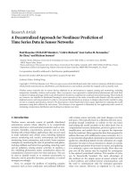
Example 1.2 (Canadian lynx data) This data set consists of the annual
fur returns of lynx at auction in London by the Hudson Bay Company for
the period 1821–1934, as listed by Elton and Nicolson (1942). It is a proxy
of the annual numbers of the Canadian lynx trapped in the Mackenzie
River district of northwest Canada and reflects to some extent the population size of the lynx in the Mackenzie River district. Hence, it helps us
to study the population dynamics of the ecological system in that area.
Indeed, if the proportion of the number of lynx being caught to the population size remains approximately constant, after logarithmic transforms,
the differences between the observed data and the population sizes remain
approximately constant. For further background information on this data


1.1 Examples of Time Series

3

Number of trapped lynx
•
3.5

•
•

•

•
•

•
3.0
2.5

•
•

•
•

••

•

•

•

•

•

•
•

•

•

•
•

•

••

•

•

•

•

•
•

•

•

•
•

•
•

•

•

•

•

•

•

•

•
•

•

•

•

•

•

•
•

••

••

•

•

•
•

•
2.0

• •
•
• •

• •

•

•

•

•
•• •

•

•

•

•

•

•
•

•

•

•
•

20

••

•
•

•
0

•

• •

•

•

•

••

•

•

•

•

•

•
•

•

•
•

•

•
40

60

80

100

FIGURE 1.2. Time series for the number (on log10 scale) of lynx trapped in the
MacKenzie River district over the period 1821–1934.

set, we refer to §7.2 of Tong (1990). Figure 1.2 depicts the time series plot
of
Xt = log10 (number of lynx trapped in year 1820 + t),

t = 1, 2, · · · , 114.

The periodic fluctuation displayed in this time series has profoundly influenced ecological theory. The data set has been constantly used to examine
such concepts as “balance-of-nature”, predator and prey interaction, and
food web dynamics, for example, see Stenseth et al. (1999) and the references therein.
Example 1.3 (Interest rate data) Short-term risk-free interest rates play
a fundamental role in financial markets. They are directly related to consumer spending, corporate earnings, asset pricing, inflation, and the overall
economy. They are used by financial institutions and individual investors
to hedge the risks of portfolios. There is a vast amount of literature on interest rate dynamics, see, for example, Duffie (1996) and Hull (1997). This
example concerns the yields of the three-month, six-month, and twelvemonth Treasury bills from the secondary market rates (on Fridays). The
secondary market rates are annualized using a 360-day year of bank interest and quoted on a discount basis. The data consist of 2,386 weekly
observations from July 17, 1959 to September 24, 1999, and are presented
in Figure 1.3. The data were previously analyzed by Andersen and Lund


4

1. Introduction

5

10

15

Yields of 3-month Treasury bills

0

500

1000
(a)

1500

2000

2

4

6

8

10

12

14

16

Yields of 6-month Treasury bills

0

500

1000
(b)

1500

2000

4

6

8

10

12

14

Yields of 12-month Treasury bills

0

500

1000
(c)

1500

2000

FIGURE 1.3. Yields of Treasury bills from July 17, 1959 to December 31, 1999
(source: Federal Reserve): (a) Yields of three-month Treasury bills; (b) yields of
six-month Treasury bills; and (c) yields of twelve-month Treasury bills.


1.1 Examples of Time Series

5

4.5

5.0

5.5

6.0

6.5

7.0

The Standard and Poor’s 500 Index

0

2000

4000

6000

FIGURE 1.4. The Standard and Poor’s 500 Index from January 3, 1972 to December 31, 1999 (on the natural logarithm scale).

(1997) and Gallant and Tauchen (1997), among others. This is a multivariate time series. As one can see in Figure 1.3, they exhibit similar structures
and are highly correlated. Indeed, the correlation coefficients between the
yields of three-month and six-month and three-month and twelve-month
Treasury bills are 0.9966 and 0.9879, respectively. The correlation matrix
among the three series is as follows:


1.0000 0.9966 0.9879
 0.9966 1.0000 0.9962  .
0.9879 0.9962 1.0000
Example 1.4 (The Standard and Poor’s 500 Index) The Standard and
Poor’s 500 index (S&P 500) is a value-weighted index based on the prices
of the 500 stocks that account for approximately 70% of the total U.S.
equity market capitalization. The selected companies tend to be the leading companies in leading industries within the U.S. economy. The index is
a market capitalization-weighted index (shares outstanding multiplied by
stock price)—the weighted average of the stock price of the 500 companies. In 1968, the S&P 500 became a component of the U.S. Department

of Commerce’s Index of Leading Economic Indicators, which are used to
gauge the health of the U.S. economy. It serves as a benchmark of stock
market performance against which the performance of many mutual funds
is compared. It is also a useful financial instrument for hedging the risks


6

1. Introduction

Avg. Level of Sulfur Dioxide

0

150

200

20

250

40

300

60

350

80

400

450

100

Number of Hospital Admissions

0

200

400
(a)

600

0

400
(b)

600

Avg. Level of Resp. Particulates

20

20

40

40

60

60

80

80

100

120

100

140

120

160

Avg. Level of Nitrogen Dioxide

200

0

200

400
(c)

600

0

200

400
(d)

600

FIGURE 1.5. Time series plots for the environmental data collected in Hong
Kong between January 1, 1994 and December 31, 1995: (a) number of hospital
admissions for circulatory and respiratory problems; (b) the daily average level
of sulfur dioxide; (c) the daily average level of nitrogen dioxide; and (d) the daily
average level of respirable suspended particulates.

of market portfolios. The S&P 500 began in 1923 when the Standard and
Poor’s Company introduced a series of indices, which included 233 companies and covered 26 industries. The current S&P 500 Index was introduced
in 1957. Presented in Figure 1.4 are the 7,076 observations of daily closing prices of the S&P 500 Index from January 3, 1972 to December 31,
1999. The logarithm transform has been applied so that the difference is
proportional to the percentage of investment return.

1.1 Examples of Time Series

7

Example 1.5 (An environmental data set) The environmental condition
plays a role in public health. There are many factors that are related to
the quality of air that may affect human circulatory and respiratory systems. The data set used here (Figure 1.5) comprises daily measurements of
pollutants and other environmental factors in Hong Kong between January
1, 1994 and December 31, 1995 (courtesy of Professor T.S. Lau). We are
interested in studying the association between the level of pollutants and
other environmental factors and the number of total daily hospital admissions for circulatory and respiratory problems. Among pollutants that were
measured are sulfur dioxide, nitrogen dioxide, and respirable suspended
particulates (in µg/m3 ). The correlation between the variables nitrogen
dioxide and particulates is quite high (0.7820). However, the correlation
between sulfur dioxide and nitrogen dioxide is not very high (0.4025). The
correlation between sulfur dioxide and respirable particulates is even lower
(0.2810). This example distinguishes itself from Example 1.3 in which the
interest mainly focuses on the study of cause and effect.
Example 1.6 (Signal processing—deceleration during car crashes) Time
series often appear in signal processing. As an example, we consider the
signals from crashes of vehicles. Airbag deployment during a crash is accomplished by a microprocessor-based controller performing an algorithm
on the digitized output of an accelerometer. The accelerometer is typically
mounted in the passenger compartment of the vehicle. It experiences decelerations of varying magnitude as the vehicle structure collapses during a
crash impact. The observed data in Figure 1.6 (courtesy of Mr. Jiyao Liu)
are the time series of the acceleration (relative to the driver) of the vehicle, observed at 1.25 milliseconds per sample. During normal driving, the
acceleration readings are very small. When vehicles are crashed or driven
on very rough and bumpy roads, the readings are much higher, depending on the severity of the crashes. However, not all such crashes activate
airbags. Federal standards define minimum requirements of crash conditions (speed and barrier types) under which an airbag should be deployed.
Automobile manufacturers institute additional requirements for the airbag

system. Based on empirical experiments using dummies, it is determined
whether a crash needs to trigger an airbag, depending on the severity of
injuries. Furthermore, for those deployment events, the experiments determine the latest time (required time) to trigger the airbag deployment
device. Based on the current and recent readings, dynamical decisions are
made on whether or not to deploy airbags.
These examples are, of course, only a few of the multitude of time series data existing in astronomy, biology, economics, finance, environmental
studies, engineering, and other areas. More examples will be introduced
later. The goal of this book is to highlight useful techniques that have
been developed to draw inferences from data, and we focus mainly on non-