Structure preserving algorithms for oscillatory differential equations II

Xinyuan Wu · Kai Liu
Wei Shi

Structure-Preserving
Algorithms
for Oscillatory
Differential
Equations II


Structure-Preserving Algorithms for Oscillatory
Differential Equations II


Xinyuan Wu Kai Liu Wei Shi
•

•

Structure-Preserving
Algorithms for Oscillatory
Differential Equations II

123


Wei Shi
Nanjing Tech University
Nanjing
China

Xinyuan Wu
Department of Mathematics
Nanjing University
Nanjing
China
Kai Liu
Nanjing University of Finance
and Economics
Nanjing
China

ISBN 978-3-662-48155-4
DOI 10.1007/978-3-662-48156-1

ISBN 978-3-662-48156-1

(eBook)

Jointly published with Science Press, Beijing, China
ISBN: 978-7-03-043918-5 Science Press, Beijing
Library of Congress Control Number: 2015950922
Springer Heidelberg New York Dordrecht London
© Springer-Verlag Berlin Heidelberg and Science Press, Beijing, China 2015
This work is subject to copyright. All rights are reserved by the Publishers, whether the whole or part
of the material is concerned, specifically the rights of translation, reprinting, reuse of illustrations,
recitation, broadcasting, reproduction on microfilms or in any other physical way, and transmission
or information storage and retrieval, electronic adaptation, computer software, or by similar or dissimilar
methodology now known or hereafter developed.
The use of general descriptive names, registered names, trademarks, service marks, etc. in this
publication does not imply, even in the absence of a specific statement, that such names are exempt from

the relevant protective laws and regulations and therefore free for general use.
The publishers, the authors and the editors are safe to assume that the advice and information in this
book are believed to be true and accurate at the date of publication. Neither the publishers nor the
authors or the editors give a warranty, express or implied, with respect to the material contained herein or
for any errors or omissions that may have been made.
Printed on acid-free paper
Springer-Verlag GmbH Berlin Heidelberg is part of Springer Science+Business Media
(www.springer.com)


This monograph is dedicated to Prof. Kang
Feng on the thirtieth anniversary of his
pioneering study on symplectic algorithms.

His profound work, which opened up a rich
new field of research, is of great importance
to numerical mathematics in China, and the
influence of his seminal contributions has
spread throughout the world.


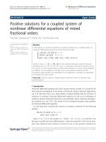
2014 Nanjing Workshop on Structure-Preserving Algorithms for Differential Equations (Nanjing,
November 29, 2014)


Preface

Numerical integration of differential equations, as an essential tool for investigating
the qualitative behaviour of the physical universe, is a very active research area
since large-scale science and engineering problems are often modelled by systems

of ordinary and partial differential equations, whose analytical solutions are usually
unknown even when they exist. Structure preservation in numerical differential
equations, known also as geometric numerical integration, has emerged in the last
three decades as a central topic in numerical mathematics. It has been realized that
an integrator should be designed to preserve as much as possible the
(physical/geometric) intrinsic properties of the underlying problem. The design and
analysis of numerical methods for oscillatory systems is an important problem that
has received a great deal of attention in the last few years. We seek to explore new
efficient classes of methods for such problems, that is high accuracy at low cost.
The recent growth in the need of geometric numerical integrators has resulted in the
development of numerical methods that can systematically incorporate the structure
of the original problem into the numerical scheme. The objective of this sequel to
our previous monograph, which was entitled “Structure-Preserving Algorithms for
Oscillatory Differential Equations”, is to study further structure-preserving integrators for multi-frequency oscillatory systems that arise in a wide range of fields
such as astronomy, molecular dynamics, classical and quantum mechanics, electrical engineering, electromagnetism and acoustics. In practical applications, such
problems can often be modelled by initial value problems of second-order differential equations with a linear term characterizing the oscillatory structure. As a
matter of fact, this extended volume is a continuation of the previous volume of our
monograph and presents the latest research advances in structure-preserving algorithms for multi-frequency oscillatory second-order differential equations. Most
of the materials of this new volume are drawn from very recent published research
work in professional journals by the research group of the authors.
Chapter 1 analyses in detail the matrix-variation-of-constants formula which
gives significant insight into the structure of the solution to the multi-frequency and
multidimensional oscillatory problem. It is known that the Störmer–Verlet formula

vii


viii

Preface

is a very popular numerical method for solving differential equations. Chapter 2
presents novel improved multi-frequency and multidimensional Störmer–Verlet
formulae. These methods are applied to solve four significant problems. For
structure-preserving integrators in differential equations, another related area of
increasing importance is the computation of highly oscillatory problems. Therefore,
Chap. 3 explores improved Filon-type asymptotic methods for highly oscillatory
differential equations. In recent years, various energy-preserving methods have
been developed, such as the discrete gradient method and the average vector field
(AVF) method. In Chap. 4, we consider efficient energy-preserving integrators
based on the AVF method for multi-frequency oscillatory Hamiltonian systems. An
extended discrete gradient formula for multi-frequency oscillatory Hamiltonian
systems is introduced in Chap. 5. It is known that collocation methods for ordinary
differential equations have a long history. Thus, in Chap. 6, we pay attention to
trigonometric Fourier collocation methods with arbitrary degrees of accuracy in
preserving some invariants for multi-frequency oscillatory second-order ordinary
differential equations. Chapter 7 analyses the error bounds for explicit ERKN
integrators for systems of multi-frequency oscillatory second-order differential
equations. Chapter 8 contains an analysis of the error bounds for two-step extended
Runge–Kutta–Nyström-type (TSERKN) methods. Symplecticity is an important
characteristic property of Hamiltonian systems and it is worthwhile to investigate
higher order symplectic methods. Therefore, in Chap. 9, we discuss high-accuracy
explicit symplectic ERKN integrators. Chapter 10 is concerned with
multi-frequency adapted Runge–Kutta–Nyström (ARKN) integrators for general
multi-frequency and multidimensional oscillatory second-order initial value problems. Butcher’s theory of trees is widely used in the study of Runge–Kutta and
Runge–Kutta–Nyström methods. Chapter 11 develops a simplified tricoloured tree
theory for the order conditions for ERKN integrators and the results presented in
this chapter are an important step towards an efficient theory of this class of
schemes. Structure-preserving algorithms for multi-symplectic Hamiltonian PDEs
are of great importance in numerical simulations. Chapter 12 focuses on general

approach to deriving local energy-preserving integrators for multi-symplectic
Hamiltonian PDEs.
The presentation of this volume is characterized by mathematical analysis,
providing insight into questions of practical calculation, and illuminating numerical
simulations. All the integrators presented in this monograph have been tested and
verified on multi-frequency oscillatory problems from a variety of applications to
observe the applicability of numerical simulations. They seem to be more efficient
than the existing high-quality codes in the scientific literature.
The authors are grateful to all their friends and colleagues for their selfless help
during the preparation of this monograph. Special thanks go to John Butcher of The
University of Auckland, Christian Lubich of Universität Tübingen, Arieh Iserles of
University of Cambridge, Reinout Quispel of La Trobe University, Jesus Maria
Sanz-Serna of Universidad de Valladolid, Peter Eris Kloeden of Goethe–
Universität, Elizabeth Louise Mansfield of University of Kent, Maarten de Hoop of
Purdue University, Tobias Jahnke of Karlsruher Institut für Technologie (KIT),


Preface

ix

Achim Schädle of Heinrich Heine University Düsseldorf and Jesus Vigo-Aguiar of
Universidad de Salamanca for their encouragement.
The authors are also indebted to many friends and colleagues for reading the
manuscript and for their valuable suggestions. In particular, the authors take this
opportunity to express their sincere appreciation to Robert Peng Kong Chan of The
University of Auckland, Qin Sheng of Baylor University, Jichun Li of University of
Nevada Las Vegas, Adrian Turton Hill of Bath University, Choi-Hong Lai of
University of Greenwich, Xiaowen Chang of McGill University, Jianlin Xia of
Purdue University, David McLaren of La Trobe University, Weixing Zheng and

Zuhe Shen of Nanjing University.
Sincere thanks also go to the following people for their help and support in
various forms: Cheng Fang, Peiheng Wu, Jian Lü, Dafu Ji, Jinxi Zhao, Liangsheng
Luo, Zhihua Zhou, Zehua Xu, Nanqing Ding, Guofei Zhou, Yiqian Wang,
Jiansheng Geng, Weihua Huang, Jiangong You, Hourong Qin, Haijun Wu,
Weibing Deng, Rong Shao, Jiaqiang Mei, Hairong Xu, Liangwen Liao and Qiang
Zhang of Nanjing University, Yaolin Jiang of Xi’an Jiao Tong University,
Yongzhong Song, Jinru Chen and Yushun Wang of Nanjing Normal University,
Xinru Wang of Nanjing Medical University, Mengzhao Qin, Geng Sun, Jialin
Hong, Zaijiu Shang and Yifa Tang of Chinese Academy of Sciences, Guangda Hu
of University of Science and Technology Beijing, Jijun Liu, Zhizhong Sun and
Hongwei Wu of Southeast University, Shoufo Li, Aiguo Xiao and Liping Wen of
Xiang Tan University, Chuanmiao Chen of Hunan Normal University, Siqing Gan
of Central South University, Chengjian Zhang and Chengming Huang of Huazhong
University of Science and Technology, Shuanghu Wang of the Institute of Applied
Physics and Computational Mathematics, Beijing, Yuhao Cong of Shanghai
University, Hongjiong Tian of Shanghai Normal University, Yongkui Zou of Jilin
University, Jingjun Zhao of Harbin Institute of Technology, Qin Ni and Chunwu
Wang of Nanjing University of Aeronautics and Astronautics, Guoqing Liu, and
Hao Cheng of Nanjing Tech University, Hongyong Wang of Nanjing University of
Finance and Economics, Theodoros Kouloukas of La Trobe University, Anders
Christian Hansen, Amandeep Kaur and Virginia Mullins of University of
Cambridge, Shixiao Wang of The University of Auckland, Qinghong Li of
Chuzhou University, Yonglei Fang of Zaozhuang University, Fan Yang, Xianyang
Zeng and Hongli Yang of Nanjing Institute of Technology, Jiyong Li of Hebei
Normal University, Bin Wang of Qufu Normal University, Xiong You of Nanjing
Agricultural University, Xin Niu of Hefei University, Hua Zhao of Beijing Institute
of Tracking and Tele Communication Technology, Changying Liu, Lijie Mei,
Yuwen Li, Qihua Huang, Jun Wu, Lei Wang, Jinsong Yu, Guohai Yang and
Guozhong Hu.

The authors would like to thank Kai Hu, Ji Luo and Tianren Sun for their help
with the editing, the editorial and production group of the Science Press, Beijing
and Springer-Verlag, Heidelberg.


x

Preface

The authors also thank their family members for their love and support
throughout all these years.
The work on this monograph was supported in part by the Natural Science
Foundation of China under Grants 11271186, by NSFC and RS International
Exchanges Project under Grant 113111162, by the Specialized Research
Foundation for the Doctoral Program of Higher Education under Grant
20100091110033 and 20130091110041, by the 985 Project at Nanjing University
under Grant 9112020301, and by the Priority Academic Program Development of
Jiangsu Higher Education Institutions.
Nanjing, China

Xinyuan Wu
Kai Liu
Wei Shi


Contents

1

2

Matrix-Variation-of-Constants Formula . . . . . . . . . . . . . . . .
1.1 Multi-frequency and Multidimensional Problems. . . . . . .
1.2 Matrix-Variation-of-Constants Formula . . . . . . . . . . . . .
1.3 Towards Classical Runge-Kutta-Nyström Schemes . . . . .
1.4 Towards ARKN Schemes and ERKN Integrators . . . . . .
1.4.1 ARKN Schemes . . . . . . . . . . . . . . . . . . . . . . .
1.4.2 ERKN Integrators . . . . . . . . . . . . . . . . . . . . . .
1.5 Towards Two-Step Multidimensional ERKN Methods . . .
1.6 Towards AAVF Methods for Multi-frequency Oscillatory
Hamiltonian Systems . . . . . . . . . . . . . . . . . . . . . . . . . .
1.7 Towards Filon-Type Methods for Multi-frequency Highly
Oscillatory Systems . . . . . . . . . . . . . . . . . . . . . . . . . . .
1.8 Towards ERKN Methods for General Second-Order
Oscillatory Systems . . . . . . . . . . . . . . . . . . . . . . . . . . .
1.9 Towards High-Order Explicit Schemes for Hamiltonian
Nonlinear Wave Equations . . . . . . . . . . . . . . . . . . . . . .
1.10 Conclusions and Discussions . . . . . . . . . . . . . . . . . . . .
References. . . . . . . . . . . . . . . . . . . . . . . . . . . . . . . . . . . . . .
Improved Störmer–Verlet Formulae with Applications . . .
2.1 Motivation . . . . . . . . . . . . . . . . . . . . . . . . . . . . . . .
2.2 Two Improved Störmer–Verlet Formulae . . . . . . . . . .
2.2.1 Improved Störmer–Verlet Formula 1 . . . . . . .
2.2.2 Improved Störmer–Verlet Formula 2 . . . . . . .
2.3 Stability and Phase Properties . . . . . . . . . . . . . . . . . .
2.4 Applications . . . . . . . . . . . . . . . . . . . . . . . . . . . . . .
2.4.1 Application 1: Time-Independent Schrödinger
Equations . . . . . . . . . . . . . . . . . . . . . . . . . .
2.4.2 Application 2: Non-linear Wave Equations . . .
2.4.3 Application 3: Orbital Problems . . . . . . . . . .

2.4.4 Application 4: Fermi–Pasta–Ulam Problem. . .

.
.
.
.
.
.
.
.

.
.
.
.
.
.
.
.

.
.
.
.
.
.
.
.

.

.
.
.
.
.
.
.

1
1
3
8
9
9
10
11

....

13

....

14

....

16

....

....
....

17
18
20

.
.
.
.
.
.
.

.
.
.
.
.
.
.

.
.
.
.
.
.
.

.
.
.
.
.
.
.

.
.
.
.
.
.
.

.
.
.
.
.
.
.

23
23
26
26
29

31
33

.
.
.
.

.
.
.
.

.
.
.
.

.
.
.
.

.
.
.
.

.
.

.
.

34
35
37
40

xi


xii

Contents

2.5

3

4

5

Coupled Conditions for Explicit Symplectic
and Symmetric Multi-frequency ERKN Integrators
for Multi-frequency Oscillatory Hamiltonian Systems . .
2.5.1 Towards Coupled Conditions for Explicit
Symplectic and Symmetric Multi-frequency
ERKN Integrators . . . . . . . . . . . . . . . . . . . . .
2.5.2 The Analysis of Combined Conditions

for SSMERKN Integrators for Multi-frequency
and Multidimensional Oscillatory Hamiltonian
Systems . . . . . . . . . . . . . . . . . . . . . . . . . . . .
2.6 Conclusions and Discussions . . . . . . . . . . . . . . . . . . .
References. . . . . . . . . . . . . . . . . . . . . . . . . . . . . . . . . . . . .
Improved Filon-Type Asymptotic Methods for Highly
Oscillatory Differential Equations . . . . . . . . . . . . . . .
3.1 Motivation . . . . . . . . . . . . . . . . . . . . . . . . . . . .
3.2 Improved Filon-Type Asymptotic Methods. . . . . .
3.2.1 Oscillatory Linear Systems . . . . . . . . . . .
3.2.2 Oscillatory Nonlinear Systems . . . . . . . .
3.3 Practical Methods and Numerical Experiments . . .
3.4 Conclusions and Discussions . . . . . . . . . . . . . . .
References. . . . . . . . . . . . . . . . . . . . . . . . . . . . . . . . .

.....

42

.....

43

.....
.....
.....

44
48
49

.
.
.
.
.
.
.
.

.
.
.
.
.
.
.
.

.
.
.
.
.
.
.
.

.
.

.
.
.
.
.
.

.
.
.
.
.
.
.
.

53
53
54
56
59
61
66
67

Efficient Energy-Preserving Integrators for Multi-frequency
Oscillatory Hamiltonian Systems . . . . . . . . . . . . . . . . . . . . .
4.1 Motivation . . . . . . . . . . . . . . . . . . . . . . . . . . . . . . . . .
4.2 Preliminaries . . . . . . . . . . . . . . . . . . . . . . . . . . . . . . .
4.3 The Derivation of the AAVF Formula . . . . . . . . . . . . . .

4.4 Some Properties of the AAVF Formula . . . . . . . . . . . . .
4.4.1 Stability and Phase Properties . . . . . . . . . . . . . .
4.4.2 Other Properties . . . . . . . . . . . . . . . . . . . . . . .
4.5 Some Integrators Based on AAVF Formula . . . . . . . . . .
4.6 Numerical Experiments . . . . . . . . . . . . . . . . . . . . . . . .
4.7 Conclusions . . . . . . . . . . . . . . . . . . . . . . . . . . . . . . . .
References. . . . . . . . . . . . . . . . . . . . . . . . . . . . . . . . . . . . . .

.
.
.
.
.
.
.
.
.
.
.

.
.
.
.
.
.
.
.
.
.

.

.
.
.
.
.
.
.
.
.
.
.

.
.
.
.
.
.
.
.
.
.
.

69
69
71
73

77
77
79
83
87
91
92

...
...
...

95
95
98

...

100

...

104

.
.
.
.
.
.

.
.

.
.
.
.
.
.
.
.

.
.
.
.
.
.
.
.

.
.
.
.
.
.
.
.

An Extended Discrete Gradient Formula for Multi-frequency
Oscillatory Hamiltonian Systems . . . . . . . . . . . . . . . . . . . . . .
5.1 Motivation . . . . . . . . . . . . . . . . . . . . . . . . . . . . . . . . . .
5.2 Preliminaries . . . . . . . . . . . . . . . . . . . . . . . . . . . . . . . .
5.3 An Extended Discrete Gradient Formula
Based on ERKN Integrators . . . . . . . . . . . . . . . . . . . . . .
5.4 Convergence of the Fixed-Point Iteration
for the Implicit Scheme . . . . . . . . . . . . . . . . . . . . . . . . .


Contents

xiii

5.5 Numerical Experiments . . . . . . . . . . . . . . . . . . . . . . . . . . . .
5.6 Conclusions . . . . . . . . . . . . . . . . . . . . . . . . . . . . . . . . . . . .
References. . . . . . . . . . . . . . . . . . . . . . . . . . . . . . . . . . . . . . . . . .
6

7

8

Trigonometric Fourier Collocation Methods
for Multi-frequency Oscillatory Systems. . . . . . . . . . . . . . . .
6.1 Motivation . . . . . . . . . . . . . . . . . . . . . . . . . . . . . . . . .
6.2 Local Fourier Expansion . . . . . . . . . . . . . . . . . . . . . . .
6.3 Formulation of TFC Methods . . . . . . . . . . . . . . . . . . . .
6.3.1 The Calculation of I1;j ; I2;j . . . . . . . . . . . . . . . .
6.3.2 Discretization . . . . . . . . . . . . . . . . . . . . . . . . .

6.3.3 The TFC Methods. . . . . . . . . . . . . . . . . . . . . .
6.4 Properties of the TFC Methods . . . . . . . . . . . . . . . . . . .
6.4.1 The Order . . . . . . . . . . . . . . . . . . . . . . . . . . .
6.4.2 The Order of Energy Preservation and Quadratic
Invariant Preservation . . . . . . . . . . . . . . . . . . .
6.4.3 Convergence Analysis of the Iteration . . . . . . . .
6.4.4 Stability and Phase Properties . . . . . . . . . . . . . .
6.5 Numerical Experiments . . . . . . . . . . . . . . . . . . . . . . . .
6.6 Conclusions and Discussions . . . . . . . . . . . . . . . . . . . .
References. . . . . . . . . . . . . . . . . . . . . . . . . . . . . . . . . . . . . .

109
114
114

.
.
.
.
.
.
.
.
.

.
.
.
.
.

.
.
.
.

.
.
.
.
.
.
.
.
.

.
.
.
.
.
.
.
.
.

117
117
120
121
122

124
125
128
129

.
.
.
.
.
.

.
.
.
.
.
.

.
.
.
.
.
.

.
.
.
.

.
.

130
133
135
137
146
146

.
.
.
.
.
.

.
.
.
.
.
.

149
149
150
152
154
155

Error Bounds for Explicit ERKN Integrators
for Multi-frequency Oscillatory Systems. . . . . . . . . . . . . . . . . .
7.1 Motivation . . . . . . . . . . . . . . . . . . . . . . . . . . . . . . . . . . .
7.2 Preliminaries for Explicit ERKN Integrators . . . . . . . . . . . .
7.2.1 Explicit ERKN Integrators and Order Conditions . .
7.2.2 Stability and Phase Properties . . . . . . . . . . . . . . . .
7.3 Preliminary Error Analysis . . . . . . . . . . . . . . . . . . . . . . . .
7.3.1 Three Elementary Assumptions
and a Gronwall’s Lemma . . . . . . . . . . . . . . . . . . .
7.3.2 Residuals of ERKN Integrators . . . . . . . . . . . . . . .
7.4 Error Bounds . . . . . . . . . . . . . . . . . . . . . . . . . . . . . . . . .
7.5 An Explicit Third Order Integrator with Minimal Dispersion
Error and Dissipation Error . . . . . . . . . . . . . . . . . . . . . . .
7.6 Numerical Experiments . . . . . . . . . . . . . . . . . . . . . . . . . .
7.7 Conclusions . . . . . . . . . . . . . . . . . . . . . . . . . . . . . . . . . .
References. . . . . . . . . . . . . . . . . . . . . . . . . . . . . . . . . . . . . . . .

..
..
..

155
156
159

.
.
.
.

.
.
.
.

166
169
173
173

Error Analysis of Explicit TSERKN Methods for Highly
Oscillatory Systems . . . . . . . . . . . . . . . . . . . . . . . . . . . .
8.1 Motivation . . . . . . . . . . . . . . . . . . . . . . . . . . . . . .
8.2 The Formulation of the New Method. . . . . . . . . . . .
8.3 Error Analysis . . . . . . . . . . . . . . . . . . . . . . . . . . .

.
.
.
.

.
.
.
.

175
175
176

183

.
.
.
.

.
.
.
.

.
.
.
.

.
.
.
.

.
.
.
.


xiv

Contents

8.4 Stability and Phase Properties .
8.5 Numerical Experiments . . . . .
8.6 Conclusions . . . . . . . . . . . . .
References. . . . . . . . . . . . . . . . . . .
9

.
.
.
.

.
.
.
.

.
.
.
.

.
.
.
.

.
.

.
.

.
.
.
.

.
.
.
.

.
.
.
.

.
.
.
.

.
.
.
.

.
.

.
.

.
.
.
.

.
.
.
.

.
.
.
.

Highly Accurate Explicit Symplectic ERKN Methods
for Multi-frequency Oscillatory Hamiltonian Systems .
9.1 Motivation . . . . . . . . . . . . . . . . . . . . . . . . . . . .
9.2 Preliminaries . . . . . . . . . . . . . . . . . . . . . . . . . .
9.3 Explicit Symplectic ERKN Methods of Order Five
with Some Small Residuals . . . . . . . . . . . . . . . .
9.4 Numerical Experiments . . . . . . . . . . . . . . . . . . .
9.5 Conclusions and Discussions . . . . . . . . . . . . . . .
References. . . . . . . . . . . . . . . . . . . . . . . . . . . . . . . . .

.
.

.
.

.
.
.
.

.
.
.
.

186
188
191
192

.........
.........
.........

193
193
194

.
.
.
.

.
.
.
.

196
204
208
208

...
...

211
211

...

212

...
...

214
215

.
.
.

.

.
.
.
.

.
.
.
.

220
222
225
227

.
.
.
.
.
.

.
.
.
.
.
.

.
.
.
.
.
.

229
229
231
233
233
234

...

235

.
.
.
.
.

236
238
238
242
245

.
.
.
.

.
.
.
.

.
.
.
.

.
.
.
.

.
.
.
.

.
.
.
.

.
.
.
.

.
.
.
.

.
.
.
.

10 Multidimensional ARKN Methods for General
Multi-frequency Oscillatory Second-Order IVPs . . . . . . . . . . .
10.1 Motivation . . . . . . . . . . . . . . . . . . . . . . . . . . . . . . . . . .
10.2 Multidimensional ARKN Methods and the Corresponding
Order Conditions . . . . . . . . . . . . . . . . . . . . . . . . . . . . .
10.3 ARKN Methods for General Multi-frequency
and Multidimensional Oscillatory Systems . . . . . . . . . . . .
10.3.1 Construction of Multidimensional ARKN Methods
10.3.2 Stability and Phase Properties of Multidimensional
ARKN Methods . . . . . . . . . . . . . . . . . . . . . . . .
10.4 Numerical Experiments . . . . . . . . . . . . . . . . . . . . . . . . .
10.5 Conclusions and Discussions . . . . . . . . . . . . . . . . . . . . .
References. . . . . . . . . . . . . . . . . . . . . . . . . . . . . . . . . . . . . . .
11 A Simplified Nyström-Tree Theory for ERKN Integrators

Solving Oscillatory Systems . . . . . . . . . . . . . . . . . . . . . . . . . .
11.1 Motivation . . . . . . . . . . . . . . . . . . . . . . . . . . . . . . . . . .
11.2 ERKN Methods and Related Issues . . . . . . . . . . . . . . . . .
11.3 Higher Order Derivatives of Vector-Valued Functions . . . .
11.3.1 Taylor Series of Vector-Valued Functions . . . . . .
11.3.2 Kronecker Inner Product . . . . . . . . . . . . . . . . . .
11.3.3 The Higher Order Derivatives and Kronecker
Inner Product . . . . . . . . . . . . . . . . . . . . . . . . . .
11.3.4 A Definition Associated with the Elementary
Differentials . . . . . . . . . . . . . . . . . . . . . . . . . . .
11.4 The Set of Simplified Special Extended Nyström Trees . . .
11.4.1 Tree Set SSENT and Related Mappings . . . . . . . .
11.4.2 The Set SSENT and the Set of Classical SN-Trees
11.4.3 The Set SSENT and the Set SENT . . . . . . . . . . .

.
.
.
.

.
.
.
.

.
.
.
.

.
.
.
.

.
.
.
.
.

.
.
.
.
.


Contents

11.5 B-series and Order Conditions
11.5.1 B-series . . . . . . . . . .
11.5.2 Order Conditions . . .
11.6 Conclusions and Discussions .
References. . . . . . . . . . . . . . . . . . .

xv

.
.

.
.
.

.
.
.
.
.

.
.
.
.
.

.
.
.
.
.

.
.
.
.
.

.
.

.
.
.

.
.
.
.
.

.
.
.
.
.

.
.
.
.
.

.
.
.
.
.

.
.

.
.
.

.
.
.
.
.

.
.
.
.
.

.
.
.
.
.

.
.
.
.
.

.
.

.
.
.

.
.
.
.
.

.
.
.
.
.

.
.
.
.
.

.
.
.
.
.

.
.

.
.
.

.
.
.
.
.

246
247
249
251
252

..
..

255
255

..

256

..
..
..

258
258
264

..

268

..

272

..

275

..
..
..

284
289
290

Conference Photo (Appendix). . . . . . . . . . . . . . . . . . . . . . . . . . . . . . .

293

Index . . . . . . . . . . . . . . . . . . . . . . . . . . . . . . . . . . . . . . . . . . . . . . . .

295

12 General Local Energy-Preserving Integrators
for Multi-symplectic Hamiltonian PDEs . . . . . . . . . . . . . . . . . .
12.1 Motivation . . . . . . . . . . . . . . . . . . . . . . . . . . . . . . . . . . .
12.2 Multi-symplectic PDEs and Energy-Preserving Continuous
Runge–Kutta Methods . . . . . . . . . . . . . . . . . . . . . . . . . . .
12.3 Construction of Local Energy-Preserving Algorithms
for Hamiltonian PDEs . . . . . . . . . . . . . . . . . . . . . . . . . .
12.3.1 Pseudospectral Spatial Discretization . . . . . . . . . . .
12.3.2 Gauss-Legendre Collocation Spatial Discretization. .
12.4 Local Energy-Preserving Schemes for Coupled Nonlinear
Schrödinger Equations . . . . . . . . . . . . . . . . . . . . . . . . . . .
12.5 Local Energy-Preserving Schemes for 2D Nonlinear
Schrödinger Equations . . . . . . . . . . . . . . . . . . . . . . . . . . .
12.6 Numerical Experiments for Coupled Nonlinear Schrödingers
Equations. . . . . . . . . . . . . . . . . . . . . . . . . . . . . . . . . . . .
12.7 Numerical Experiments for 2D Nonlinear Schrödinger
Equations. . . . . . . . . . . . . . . . . . . . . . . . . . . . . . . . . . . .
12.8 Conclusions . . . . . . . . . . . . . . . . . . . . . . . . . . . . . . . . . .
References. . . . . . . . . . . . . . . . . . . . . . . . . . . . . . . . . . . . . . . .

.
.
.
.
.


Chapter 1

Matrix-Variation-of-Constants Formula

The first chapter presents the matrix-variation-of-constants formula which is fundamental to structure-preserving integrators for multi-frequency and multidimensional
oscillatory second-order differential equations in the current volume and the previous
volume [23] of our monograph since the formula makes it possible to incorporate
the special structure of the multi-frequency oscillatory problems into the integrators.

1.1 Multi-frequency and Multidimensional Problems
Oscillatory second-order initial value problems constitute an important category of
differential equations in pure and applied mathematics, and in applied sciences such
as mechanics, physics, astronomy, molecular dynamics and engineering. Among
traditional and typical numerical schemes for solving these kinds of problems is the
well-known Runge-Kutta-Nyström method [13], which has played an important role
since 1925 in dealing with second-order initial value problems of the conventional
form
y = f (y, y ), x ∈ [x0 , xend ],
(1.1)
y(x0 ) = y0 , y (x0 ) = y0 .
However, many systems of second-order differential equations arising in applications
have the general form
y + M y = f (y, y ), x ∈ [x0 , xend ],
y(x0 ) = y0 ,

y (x0 ) = y0 ,

(1.2)

where M ∈ Rd×d is a positive and semi-definite matrix (not necessarily diagonal nor
symmetric, in general) that implicitly contains and preserves the main frequencies of

the oscillatory problem. Here, f : Rd × Rd → Rd , with the position y(x) ∈ Rd and
© Springer-Verlag Berlin Heidelberg and Science Press, Beijing, China 2015
X. Wu et al., Structure-Preserving Algorithms for Oscillatory
Differential Equations II, DOI 10.1007/978-3-662-48156-1_1

1


2

1 Matrix-Variation-of-Constants Formula

the velocity y (x) as arguments. The system (1.2) is a multi-frequency and multidimensional oscillatory problem which exhibits pronounced oscillatory behaviour due
to the linear term M y. Among practical examples we mention the damped harmonic
oscillator, the van der Pol equation, the Liénard equation (see [10]) and the damped
wave equation. The design and analysis of numerical integrators for nonlinear oscillators is an important problem that has received a great deal of attention in the last
few years.
It is important to observe that the special case M = 0 in (1.2) reduces to the
conventional form of second-order initial value problems (1.1). Therefore, each integrator for the system (1.2) is applicable to the conventional second-order initial value
problems (1.1). Consequently, this extended volume of our monograph focuses only
on the general second-order oscillatory system (1.2).
When the function f does not contain the first derivative y , (1.2) reduces to the
special and important multi-frequency oscillatory system
y + M y = f (y), x ∈ [x0 , xend ],
y(x0 ) = y0 , y (x0 ) = y0 .

(1.3)

If M is symmetric and positive semi-definite and f (y) = −∇U (y), then with q = y,
p = y , (1.3) becomes identical to a multi-frequency and multidimensional oscillatory Hamiltonian system of the form

p = −∇q H ( p, q), p(x0 ) = p0 ,
q = ∇ p H ( p, q), q(x0 ) = q0 ,

(1.4)

with the Hamiltonian
H ( p, q) =

1
1
p p + q Mq + U (q),
2
2

(1.5)

where U (q) is a smooth potential function. The solution of the system (1.4) exhibits
nonlinear oscillations. Mechanical systems with a partitioned Hamiltonian function
yield examples of this type. It is well known that two fundamental properties of
Hamiltonian systems are:
(i) the solutions preserve the Hamiltonian H , i.e., H ( p(x), q(x)) ≡ H ( p0 , q0 ) for
any x ≥ x0 ;
(ii) the corresponding flow is symplectic, i.e., it preserves the differential 2-form
d

d pi ∧ dqi .

i=1

It is true that great advances have been made in the theory of general-purpose

methods for the numerical solution of ordinary differential equations. However, the
numerical implementation of a general-purpose method cannot respect the qualitative behaviour of a multi-frequency and multidimensional oscillatory problem. It


1.1 Multi-frequency and Multidimensional Problems

3

turns out that structure-preserving integrators are required in order to produce the
qualitative properties of the true flow of the multi-frequency oscillatory problem.
This new volume represents an attempt to extend our previous volume [23] and
presents the very recent advances in Runge-Kutta-Nyström-type (RKN-type) methods for multi-frequency oscillatory second-order initial value problems (1.2). To this
end, the following matrix-variation-of-constants formula is fundamental and plays
an important role.

1.2 Matrix-Variation-of-Constants Formula
The following matrix-variation-of-constants formula gives significant insight into
the structure of the solution to the multi-frequency and multidimensional problem
(1.2), which has motivated the formulation of multi-frequency and multidimensional
adapted Runge-Kutta-Nyström (ARKN) schemes, and multi-frequency and multidimensional extended Runge-Kutta-Nyström (ERKN) integrators, as well as classical
RKN methods.
Theorem 1.1 (Wu et al. [21]) If M ∈ Rd×d is a positive semi-definite matrix and
f : Rd × Rd → Rd in (1.2) is continuous, then the exact solution of (1.2) and its
derivative satisfy
⎧
y(x) = φ0 (x − x0 )2 M y0 + (x − x0 )φ1 (x − x0 )2 M y0
⎪
⎪
⎪
⎪

x
⎪
⎪
⎪
+
(x − ζ )φ1 (x − ζ )2 M fˆ(ζ )dζ,
⎪
⎨
x0

⎪
y (x) = − (x − x0 )Mφ1 (x − x0 )2 M y0 + φ0 (x − x0 )2 M y0
⎪
⎪
⎪
⎪
x
⎪
⎪
⎪
+
φ0 (x − ζ )2 M fˆ(ζ )dζ,
⎩

(1.6)

x0

for x0 , x ∈ (−∞, +∞), where
fˆ(ζ ) = f y(ζ ), y (ζ )

and the matrix-valued functions φ0 (M) and φ1 (M) are defined by
φ0 (M) =

∞ (−1)k M k
(−1)k M k
, φ1 (M) =
.
(2k)!
k=0
k=0 (2k + 1)!
∞

(1.7)

We notice that these matrix-valued functions reduce to the φ-functions used for
Gautschi-type trigonometric or exponential integrators in [4, 7] when M is a symmetric and positive semi-definite matrix.


4

1 Matrix-Variation-of-Constants Formula

With regard to algorithms for computing the matrix-valued functions φ0 (M) and
φ1 (M), we refer the reader to [1] and references therein.
Taking the importance of the matrix-variation-of-constants formula into account,
a brief proof is presented in a self-contained way.
Proof Multiplying both sides of the equation in formula (1.2) (using ζ for the independent variable) by (x − ζ )φ1 (x − ζ )2 M and integrating from x0 to x yields
x

(x − ζ )φ1 (x − ζ )2 M y (ζ )dζ +

x0

=

x

(x − ζ )φ1 (x − ζ )2 M M y(ζ )dζ

x0
x

(x − ζ )φ1 (x − ζ ) M fˆ(ζ )dζ.
2

x0

Applying integration by parts twice to the first term on the left-hand side gives the
first equation of (1.6) on noticing that
(x − ζ )φ1 ((x − ζ )2 M)

= −φ0 (x − ζ )2 M ,

and
φ0 (x − ζ )2 M

= (x − ζ )φ1 (x − ζ )2 M M.

Likewise, multiplying both sides of the equation in formula (1.2) by φ0 (x − ζ )2 M
and integrating from x0 to x yields

x
x0

φ0 (x − ζ )2 M y (ζ )dζ +

x
x0

φ0 (x − ζ )2 M M y(ζ )dζ =

x
x0

φ0 (x − ζ )2 M fˆ(ζ )dζ.

Integration by parts twice in the first term on the left-hand side gives the second
equation of (1.6).
Here and in the remainder of this chapter, the integral of a matrix function is
understood componentwise.
We notice that a conventional form of variation-of-constants formula in the literature (see, e.g. [3] by García-Archilla et al., [4, 5] by Hairer et al., and [7] by
Hochbruck et al.) for the special oscillatory system (1.3) is expressed by
⎧
y(x) = cos (x − x0 )Ω y0 + Ω −1 sin (x − x0 )Ω y0
⎪
⎪
⎪
⎪
x
⎪
⎪

⎪
⎪
+
Ω −1 sin (x − τ )Ω g(τ
ˆ )dτ,
⎨
x0
(1.8)
⎪
y
(x)
=
−
Ω
sin
(x
−
x
)Ω
y
+
cos
(x
−
x
)Ω
y
⎪
0
0

0
0
⎪
⎪
⎪
x
⎪
⎪
⎪
+
cos (x − τ )Ω g(τ
ˆ )dτ,
⎩
x0

ˆ ) = f y(τ ) .
where M = Ω 2 and g(τ


1.2 Matrix-Variation-of-Constants Formula

5

It is very clear that the matrix-variation-of-constants formula (1.6) for general
oscillatory systems (1.2) does not involve the decomposition of M and is different
from the conventional one for the oscillatory system (1.3) in which f is independent
of y . It is also important to avoid matrix decompositions in an integrator for multifrequency and multidimensional oscillatory systems as M is not necessarily diagonal
nor symmetric in (1.2) and the decomposition M = Ω 2 is not always feasible. Therefore, the matrix-variation-of-constants formula (1.6) without the decomposition of
matrix M has wider applications in general.
In the particular case M = ω2 Id , (1.3) becomes

y + ω2 y = f (y), x ∈ [x0 , xend ],
y(x0 ) = y0 ,

y (x0 ) = y0 ,

(1.9)

and the corresponding variation-of-constants formula is well known. That is,
⎧
y(x) = cos (x − x0 )ω y0 + ω−1 sin (x − x0 )ω y0
⎪
⎪
⎪
⎪
x
⎪
⎪
⎪
⎪
+
ω−1 sin (x − τ )ω g(τ
ˆ )dτ,
⎨
x0

⎪
y (x) = − ω sin (x − x0 )ω y0 + cos (x − x0 )ω y0
⎪
⎪
⎪

⎪
x
⎪
⎪
⎪
+
cos (x − τ )ω g(τ
ˆ )dτ.
⎩

(1.10)

x0

If M is symmetric and positive semi-definite, it is easy to see that (1.8) can be
straightforwardly obtained by formally replacing ω with Ω = M 1/2 in the formula
(1.10) as pointed out in Sect. XIII.1.2 in [5] by Hairer et al. However, it is required
to show (1.6) by a rigorous proof as M is not necessarily symmetric or diagonal and
f depends on both y and y in (1.2).
It follows from formula (1.6) of Theorem 1.1 that, for any x, μ, h ∈ R with
x, x + μh ∈ [x0 , xend ], the solution to (1.2) satisfies the following integral equations:
⎧
y(x + μh) = φ0 (μ2 V )y(x) + hμφ1 (μ2 V )y (x)
⎪
⎪
⎪
μ
⎪
⎪
⎪

⎪
(μ − ζ )φ1 (μ − ζ )2 V fˆ x + ζ h dζ,
+ h2
⎨
0

⎪
y (x + μh) = φ0 (μ2 V )y (x) − μh Mφ1 (μ2 V )y(x)
⎪
⎪
⎪
⎪
μ
⎪
⎪
⎩
φ0 (μ − ζ )2 V fˆ x + ζ h dζ,
+h

(1.11)

0

where V = h 2 M, and the d ×d matrix-valued functions φ0 (V ) and φ1 (V ) are defined
by (1.7).
It can be observed that the matrix-variation-of-constants formula (1.11) subsumes
the structure of the internal stages and updates for an extended and improved RKNtype integrator. In fact, if y(xn ) and y (xn ) are prescribed, it follows from (1.11)
that

6

1 Matrix-Variation-of-Constants Formula

⎧
y(xn + μh) = φ0 (μ2 V )y(xn ) + μhφ1 (μ2 V )y (xn )
⎪
⎪
⎪
μ
⎪
⎪
⎪
⎪
(μ − ζ )φ1 (μ − ζ )2 V fˆ(xn + hζ )dζ,
+ h2
⎨
0

⎪
y (xn + μh) = − μh Mφ1 (μ2 V )y(xn ) + φ0 (μ2 V )y (xn )
⎪
⎪
⎪
⎪
μ
⎪
⎪
⎩
φ0 (μ − ζ )2 V fˆ(xn + hζ )dζ,

+h

(1.12)

0

for 0 < μ < 1, and
⎧
y(xn + h) = φ0 (V )y(xn ) + hφ1 (V )y (xn )
⎪
⎪
⎪
⎪
1
⎪
⎪
⎪
⎪
+ h2
(1 − ζ )φ1 (1 − ζ )2 V fˆ(xn + hζ )dζ,
⎨
0

⎪
y (xn + h) = − h Mφ1 (V )y(xn ) + φ0 (V )y (xn )
⎪
⎪
⎪
⎪
1

⎪
⎪
⎪
⎩
+h
φ0 (1 − ζ )2 V fˆ(xn + hζ )dζ,

(1.13)

0

for μ = 1.
The formulae (1.12) and (1.13) suggest clearly the structure of the internal stages
and updates for an improved RKN-type integrator when they are applied to multifrequency and multidimensional oscillatory systems (1.2), respectively.
As a simple example, the trapezoidal discretization of the integrals in formula
(1.13) with a fixed stepsize h gives the implicit scheme
⎧
1 2
⎪
⎪
⎪ yn+1 = φ0 (V )yn + hφ1 (V )yn + h φ1 (V ) f (yn , yn ),
⎪
2
⎨
yn+1 = − h Mφ1 (V )yn + φ0 (V )yn
⎪
⎪
⎪
1
⎪

⎩
+ h φ0 (V ) f (yn , yn ) + f (yn+1 , yn+1 ) .
2

(1.14)

If the function f does not depend on the first derivative y , formula (1.14) reduces
to an explicit scheme
⎧
1
⎪
⎨ yn+1 = φ0 (V )yn + hφ1 (V )yn + h 2 φ1 (V ) f (yn ),
2
1
⎪
⎩y
n+1 = −h Mφ1 (V )yn + φ0 (V )yn + h φ0 (V ) f (yn ) + f (yn+1 ) ,
2

(1.15)

which was first given in [2] for the initial value problem
y + ω2 y = f (y),

y(x0 ) = y0 ,

y (x0 ) = y0 ,

where ω > 0. This means that the integrator (1.14) reduces to the Deuflhard method
in the particular case M = ω2 I .

1.2 Matrix-Variation-of-Constants Formula

7

As another example, we consider to apply the variation-of constants formula (1.6)
to high-dimensional nonlinear Hamiltonian wave equations:
u tt (X, t) = f u(X, t) + a 2 Δu(X, t), X ∈
u(X, t0 ) = ϕ1 (X ), u t (X, t0 ) = ϕ2 (X ), X ∈
where f (u) = −

dG u(X,t)
du

⊆ Rd , t > t0 ,
∪∂ ,

(1.16)

and
d

Δ=
i=1

∂2
.
∂ xi2

Applying the variation-of-constants formula (1.6) to (1.16) gives an analytical
expression for the solution of (1.16):
⎧
u(X, t) = u(X, t0 ) + (t − t0 )u t (X, t0 )
⎪
⎪
⎪
⎪
t
⎪
⎪
⎪
(t − ζ ) f u(X, ζ ) + a 2 Δu(X, ζ ) dζ,
+
⎪
⎨
t0
(1.17)
t
⎪
⎪
2
⎪
f u(X, ζ ) + a Δu(X, ζ ) dζ,
u t (X, t) = u t (X, t0 ) +
⎪
⎪
⎪
t0
⎪

⎪
⎩
X ∈ ∪∂ ,
i.e.,
⎧
u(X, t) = ϕ1 (X ) + (t − t0 )ϕ2 (X )
⎪
⎪
⎪
⎪
t
⎪
⎪
⎪
(t − ζ ) f u(X, ζ ) + a 2 Δu(X, ζ ) dζ,
+
⎪
⎨
t0

t
⎪
⎪
⎪
f u(X, ζ ) + a 2 Δu(X, ζ ) dζ,
(X,
t)
=
ϕ
(X

)
+
u
⎪
t
2
⎪
⎪
t0
⎪
⎪
⎩
X ∈ ∪∂ .

(1.18)

Under suitable assumptions it can be proved that (1.18) is consistent with Dirichlet boundary conditions, Neumann boundary conditions, and Robin boundary conditions, respectively.
Formula (1.17) for the purpose of numerical simulation can be written as


8

1 Matrix-Variation-of-Constants Formula

⎧
⎪
⎪ u(X, tn + h) = u(X, tn ) + hu t (X, tn )
⎪
⎪
⎪

1
⎪
⎪
2
⎪
+
h
(1 − ζ ) f u(X, tn + ζ h) + a 2 Δu(X, tn + ζ h) dζ,
⎪
⎪
⎪
0
⎨
u t (X, tn + h) = u t (X, tn )
⎪
⎪
1
⎪
⎪
⎪
⎪
f u(X, tn + ζ h) + a 2 Δu(X, tn + ζ h) dζ,
+
h
⎪
⎪
⎪
0
⎪
⎪

⎩ n = 0, 1, . . . ,
X ∈ ∪∂ .

(1.19)

1.3 Towards Classical Runge-Kutta-Nyström Schemes
It is well known that Nyström [13] proposed a direct approach to solving secondorder initial value problems (1.1) numerically. To show this point clearly, from the
matrix-variation-of-constants formula (1.11) with M = 0, we first give the following
integral formulae for second-order initial value problems (1.1):
⎧
2
⎪
⎪
⎨ y(xn + μh) = y(xn ) + μhy (xn ) + h
μ

⎪
⎪
⎩ y (xn + μh) = y (xn ) + h

μ

(μ − ζ )ϕ(xn + hζ ) dζ,

0

(1.20)

ϕ(xn + hζ ) dζ,

0

for 0 < μ < 1, and
⎧
⎪
2
⎪
⎪
⎨ y(xn + h) = y(xn ) + hy (xn ) + h
⎪
⎪
⎪
⎩ y (xn + h) = y (xn ) + h

1

1

(1 − ζ )ϕ(xn + hζ ) dζ,

0

(1.21)

ϕ(xn + hζ ) dζ,

0

for μ = 1, where ϕ(ν) := f y(ν), y (ν) .
Formulae (1.20) and (1.21) contain and show clearly the structure of the internal

stages and updates of a Runge-Kutta-type integrator for solving (1.1), respectively.
This suggests the classical Runge-Kutta-Nyström scheme in a quite simple and natural way in comparison to the original idea (that is, with the block vector (y , y )
considered as a new variable, (1.1) can be transformed into a first-order differential
equation of doubled dimension. Then apply Runge-Kutta methods to the first-order
differential equation, together with some simplifications). In fact, approximating
the integrals in (1.20) and (1.21) by using suitable quadrature formulae straightforwardly yields the classical Runge-Kutta-Nyström scheme (see, e.g. [6, 13]) given by
the following definition.
Definition 1.1 An s-stage Runge-Kutta-Nyström (RKN) method for the initial value
problem (1.1) is defined by


1.3 Towards Classical Runge-Kutta-Nyström Schemes

9

⎧
s
⎪
⎪
Yi = yn + ci hyn + h 2
a¯ i j f (Y j , Y j ), i = 1, . . . , s,
⎪
⎪
⎪
j=1
⎪
⎪
s
⎪
⎪

⎪
ai j f (Y j , Y j ), i = 1, . . . , s,
⎨ Yi = yn + h
j=1

s
⎪
2
⎪
⎪
=
y
+
hy
+
h
y
b¯i f (Yi , Yi ),
n+1
n
n
⎪
⎪
⎪
i=1
⎪
s
⎪
⎪
⎪

⎩ yn+1 = yn + h
bi f (Yi , Yi ),

(1.22)

i=1

or expressed equivalently by the conventional form
⎧
s
⎪
2
⎪
k
=
f
(y
+
c
hy
+
h
a¯ i j k j , yn + h
i
n
i
⎪
n
⎪
⎪

j=1
⎪
⎨
s
yn+1 = yn + hyn + h 2
b¯i ki ,
⎪
i=1
⎪
⎪
s
⎪
⎪
⎪
bi ki ,
⎩ yn+1 = yn + h

s

ai j k j ), i = 1, . . . , s,

j=1

(1.23)

i=1

where a¯ i j , ai j , b¯i , bi , ci for i, j = 1, . . . , s are real constants.
Conventionally, the RKN method (1.22) can be expressed by the following partitioned
Butcher tableau:

c1 a¯ 11 · · · a¯ 1s a11 · · · a1s
.. .. . . .. .. . . ..
. . .
. .
c A¯ A = . .
a
¯
·
·
·
a
¯
a
·
·
·
ass
c
s s1
ss s1
b¯ b
b¯1 · · · b¯s b1 · · · bs
where b¯ = (b¯1 , . . . , b¯s ) , b = (b1 , . . . , bs ) and c = (c1 , . . . , cs ) are sdimensional vectors, and A¯ = (a¯ i j ) and A = (ai j ) are s × s constant matrices.

1.4 Towards ARKN Schemes and ERKN Integrators
1.4.1 ARKN Schemes
Inheriting the internal stages of the classical RKN methods and approximating the
integrals in (1.13) by a suitable quadrature formula to modify the updates of the
classical RKN methods gives the ARKN methods for the multi-frequency and multidimensional oscillatory system (1.2).
Definition 1.2 (Wu et al. [22]) An s-stage ARKN method for numerical integration

of the multi-frequency and multidimensional oscillatory system (1.2) is defined as


10

1 Matrix-Variation-of-Constants Formula

⎧
⎪
⎪
⎪
⎪
⎪
⎪
⎪
⎪
⎪
⎪
⎪
⎪
⎪
⎪
⎪
⎪
⎨

s

a¯ i j f (Y j , Y j ) − MY j ,

Yi = yn + hci yn + h 2

i = 1, . . . , s,

j=1
s

ai j f (Y j , Y j ) − MY j ,

Yi = yn + h

i = 1, . . . , s,

j=1

s
⎪
⎪
⎪
2
⎪
yn+1 = φ0 (V )yn + hφ1 (V )yn + h
b¯i (V ) f (Yi , Yi ),
⎪
⎪
⎪
⎪
i=1
⎪
⎪

⎪
s
⎪
⎪
⎪
⎪
⎪
y
=
φ
(V
)y
−
h
Mφ
(V
)y
+
h
bi (V ) f (Yi , Yi ),
0
1
n
⎩ n+1
n

(1.24)

i=1

where a¯ i j , ai j , ci for i, j = 1, . . . , s are real constants, and the weight functions
b¯i (V ), bi (V ) for i = 1, . . . , s in the updates are matrix-valued functions of V =
h 2 M.
The ARKN scheme (1.24) can also be denoted by the Butcher tableau
a11 · · · a1s
c1 a¯ 11 · · · a¯ 1s
..
..
..
..
..
..
..
.
.
.
.
.
.
.
A
c A¯
=
as1 · · · ass
cs a¯ s1 · · · a¯ ss
¯b (V ) b (V )
b¯1 (V ) · · · b¯s (V ) b1 (V ) · · · bs (V )
It should be noticed that the internal stages of an ARKN method are exactly the
same as the classical RKN methods, but the updates have been revised in light of the
matrix-variation-of-constants formula (1.13).

A detailed analysis for a six-stage ARKN method of order five will be presented
in Chap. 10 for the case of general oscillatory second-order initial value problems
(1.2).

1.4.2 ERKN Integrators
Explicitly, the matrix-variation-of-constants formula (1.6) with fˆ(ζ ) = f y(ζ ) can
be easily applied to the special oscillatory system (1.3), as in (1.12) and (1.13). Then,
approximating the integrals in (1.12) and (1.13) using suitable quadrature formulae
leads to the following ERKN integrator for the oscillatory system (1.3).
Definition 1.3 (Wu et al. [21]) An s-stage ERKN integrator for the numerical integration of the oscillatory system (1.3) is defined by