Quantum chromodynamics at high energy
Bạn đang xem bản rút gọn của tài liệu. Xem và tải ngay bản đầy đủ của tài liệu tại đây (2.61 MB, 350 trang )
QUANTUM CHROMODYNAMICS AT HIGH ENERGY
Filling a gap in the current literature, this book is the first entirely dedicated to
high energy quantum chromodynamics (QCD) including parton saturation and the
color glass condensate (CGC). It presents groundbreaking progress on the subject and
describes many problems at the forefront of research, bringing postgraduate students,
theorists, and interested experimentalists up to date with the current state of research
in this field.
The material is presented in a pedagogical way, with numerous examples and
exercises. Discussion ranges from the quasi-classical McLerran–Venugopalan model
to the linear BFKL and nonlinear BK/JIMWLK small-x evolution equations. The
authors adopt both a theoretical and an experimental outlook, and present the physics
of strong interactions in a universal way, making it useful for physicists from various
subcommunities of high energy and nuclear physics, and applicable to processes
studied at all high energy accelerators around the world. A selection of color figures
is available online at www.cambridge.org/9780521112574.
Y u r i V . K o v c h e g o v is Professor in the Department of Physics at The Ohio
State University. He is a world leader in the field of high energy QCD. In 2006 he
was awarded The Raymond and Beverly Sackler Prize in the Physical Sciences by
Tel Aviv University for a number of groundbreaking contributions in the field. The
Balitsky–Kovchegov equation bears his name.
E u g e n e L e v i n is Professor Emeritus in the School of Physics and Astronomy at
Tel Aviv University. He is the founding father of the field of parton saturation and of
the constituent quark model. Equations and approaches that bear his name include the
Levin–Frankfurt quark-counting rules, the Gribov–Levin–Ryskin nonlinear equation,
the Levin–Tuchin solution, and the Kharzeev–Levin–Nardi approach, reflecting only
a selection of his many contributions to high energy physics.
Downloaded from Cambridge Books Online by IP 150.244.9.175 on Tue Apr 09 19:08:51 WEST 2013.
/>Cambridge Books Online © Cambridge University Press, 2013
CAMBRIDGE MONOGRAPHS ON PARTICLE PHYSICS,
NUCLEAR PHYSICS AND COSMOLOGY
General Editors: T. Ericson, P. V. Landshoff
1. K. Winter (ed.): Neutrino Physics
2. J. F. Donoghue, E. Golowich and B. R. Holstein: Dynamics of the Standard Model
3. E. Leader and E. Predazzi: An Introduction to Gauge Theories and Modern Particle Physics,
Volume 1: Electroweak Interactions, the ‘New Particles’ and the Parton Model
4. E. Leader and E. Predazzi: An Introduction to Gauge Theories and Modern Particle Physics,
Volume 2: CP-Violation, QCD and Hard Processes
5. C. Grupen: Particle Detectors
6. H. Grosse and A. Martin: Particle Physics and the Schr¨odinger Equation
7. B. Anderson: The Lund Model
8. R. K. Ellis, W. J. Stirling and B. R. Webber: QCD and Collider Physics
9. I. I. Bigi and A. I. Sanda: CP Violation
10. A. V. Manohar and M. B. Wise: Heavy Quark Physics
11. R. K. Bock, H. Grote, R. Fr¨uhwirth and M. Regler: Data Analysis Techniques for
High-Energy Physics, Second edition
12. D. Green: The Physics of Particle Detectors
13. V. N. Gribov and J. Nyiri: Quantum Electrodynamics
14. K. Winter (ed.): Neutrino Physics, Second edition
15. E. Leader: Spin in Particle Physics
16. J. D. Walecka: Electron Scattering for Nuclear and Nucleon Scattering
17. S. Narison: QCD as a Theory of Hadrons
18. J. F. Letessier and J. Rafelski: Hadrons and Quark–Gluon Plasma
19. A. Donnachie, H. G. Dosch, P. V. Landshoff and O. Nachtmann: Pomeron Physics and QCD
20. A. Hoffmann: The Physics of Synchroton Radiation
21. J. B. Kogut and M. A. Stephanov: The Phases of Quantum Chromodynamics
22. D. Green: High PT Physics at Hadron Colliders
23. K. Yagi, T. Hatsuda and Y. Miake: Quark–Gluon Plasma
24. D. M. Brink and R. A. Broglia: Nuclear Superfluidity
25. F. E. Close, A. Donnachie and G. Shaw: Electromagnetic Interactions and Hadronic
Structure
26. C. Grupen and B. A. Schwartz: Particle Detectors, Second edition
27. V. Gribov: Strong Interactions of Hadrons at High Energies
28. I. I. Bigi and A. I. Sanda: CP Violation, Second edition
29. P. Jaranowski and A. Kr´olak: Analysis of Gravitational Wave Data
30. B. L. Ioffe, V. S. Fadin and L. N. Lipatov: Quantum Chromodynamics: Perturbative and
Nonperturbative Aspects
31. J. M. Cornwall, J. Papavassiliou and D. Binosi: The Pinch Technique and its Applications to
Non-Abelian Gauge Theories
32. J. Collins: Foundations of Perturbative QCD
33. Y. V. Kovchegov and E. Levin: Quantum Chromodynamics at High Energy
Downloaded from Cambridge Books Online by IP 150.244.9.175 on Tue Apr 09 19:08:51 WEST 2013.
/>Cambridge Books Online © Cambridge University Press, 2013
QUANTUM CHROMODYNAMICS
AT HIGH ENERGY
YURI V. KOVCHEGOV
The Ohio State University, USA
EUGENE LEVIN
Tel-Aviv University, Israel
Downloaded from Cambridge Books Online by IP 150.244.9.175 on Tue Apr 09 19:08:51 WEST 2013.
/>Cambridge Books Online © Cambridge University Press, 2013
cambridge university press
Cambridge, New York, Melbourne, Madrid, Cape Town,
Singapore, S˜ao Paulo, Delhi, Mexico City
Cambridge University Press
The Edinburgh Building, Cambridge CB2 8RU, UK
Published in the United States of America by Cambridge University Press, New York
www.cambridge.org
Information on this title: www.cambridge.org/9780521112574
C
Y. V. Kovchegov and E. Levin 2012
This publication is in copyright. Subject to statutory exception
and to the provisions of relevant collective licensing agreements,
no reproduction of any part may take place without the written
permission of Cambridge University Press.
First published 2012
Printed in the United Kingdom at the University Press, Cambridge
A catalog record for this publication is available from the British Library
p.
Library of Congress Catalog in Publication data
Kovchegov, Yuri V., 1973–
Quantum chromodynamics at high energy / Yuri V. Kovchegov, Eugene Levin.
cm. – (Cambridge monographs on particle physics, nuclear physics and cosmology ; 33)
Includes bibliographical references and index.
ISBN 978-0-521-11257-4 (hardback)
1. Quantum chromodynamics. I. Levin, Eugene (Eugene M.) II. Title.
QC793.3.Q35K68 2012
539.7 548 – dc23
2012016517
ISBN 978-0-521-11257-4 Hardback
Additional resources for this publication are at www.cambridge.org/9780521112574
Cambridge University Press has no responsibility for the persistence or
accuracy of URLs for external or third-party internet websites referred to
in this publication, and does not guarantee that any content on such
websites is, or will remain, accurate or appropriate.
Downloaded from Cambridge Books Online by IP 150.244.9.175 on Tue Apr 09 19:08:51 WEST 2013.
/>Cambridge Books Online © Cambridge University Press, 2013
Contents
Preface
1
1.1
1.2
1.3
1.4
1.5
page ix
Introduction: basics of QCD perturbation theory
The QCD Lagrangian
A review of Feynman rules for QCD
1.2.1 QCD Feynman rules
Rules of light cone perturbation theory
1.3.1 QCD LCPT rules
1.3.2 Light cone wave function
Sample LCPT calculations
1.4.1 LCPT “cross-check”
1.4.2 A sample light cone wave function
Asymptotic freedom
2
2.1
2.2
Deep inelastic scattering
Kinematics, cross section, and structure functions
Parton model and Bjorken scaling
2.2.1 Warm-up: DIS on a single free quark
2.2.2 Full calculation: DIS on a proton
2.3
Space–time structure of DIS processes
2.4
Violation of Bjorken scaling;
the Dokshitzer–Gribov–Lipatov–Altarelli–Parisi evolution equation
2.4.1 Parton distributions
2.4.2 Evolution for quark distribution
2.4.3 The DGLAP evolution equations
2.4.4 Gluon–gluon splitting function∗
2.4.5 General solution of the DGLAP equations
2.4.6 Double logarithmic approximation
Further reading
Exercises
v
Downloaded from Cambridge Books Online by IP 150.244.9.175 on Tue Apr 09 19:09:14 WEST 2013.
/>Cambridge Books Online © Cambridge University Press, 2013
1
1
3
6
7
10
12
14
14
17
19
22
22
27
27
29
38
43
43
45
53
56
60
63
72
72
vi
Contents
3
3.1
3.2
3.3
Energy evolution and leading logarithm-1/x approximation in QCD
Paradigm shift
Two-gluon exchange: the Low–Nussinov pomeron
The Balitsky–Fadin–Kuraev–Lipatov evolution equation
3.3.1 Effective emission vertex
3.3.2 Virtual corrections and reggeized gluons
3.3.3 The BFKL equation
3.3.4 Solution of the BFKL equation
3.3.5 Bootstrap property of the BFKL equation∗
3.3.6 Problems of BFKL evolution: unitarity and diffusion
3.4
The nonlinear Gribov–Levin–Ryskin and Mueller–Qiu evolution equation
3.4.1 The physical picture of parton saturation
3.4.2 The GLR–MQ equation
Further reading
Exercises
74
74
76
82
83
88
92
95
103
107
112
112
115
121
121
4
4.1
4.2
Dipole approach to high parton density QCD
Dipole picture of DIS
Glauber–Gribov–Mueller multiple-rescatterings formula
4.2.1 Scattering on one nucleon
4.2.2 Scattering on many nucleons
4.2.3 Saturation picture from the GGM formula
4.3
Mueller’s dipole model
4.3.1 Dipole wave function and generating functional
4.3.2 The BFKL equation in transverse coordinate space
4.3.3 The general solution of the coordinate-space BFKL equation∗
4.4
The Balitsky–Kovchegov equation
4.5
Solution of the Balitsky–Kovchegov equation
4.5.1 Solution outside the saturation region; extended geometric scaling
4.5.2 Solution inside the saturation region; geometric scaling
4.5.3 Semiclassical solution
4.5.4 Traveling wave solution
4.5.5 Numerical solutions
4.5.6 Map of high energy QCD
4.6
The Bartels–Kwiecinski–Praszalowicz equation∗
4.7
The odderon∗
Further reading
Exercises
123
123
129
130
133
139
141
141
153
159
163
172
172
176
178
181
184
188
189
192
195
196
5
5.1
198
198
198
200
Classical gluon fields and the color glass condensate
Strong classical gluon fields: the McLerran–Venugopalan model
5.1.1 The key idea of the approach
5.1.2 Classical gluon field of a single nucleus
Downloaded from Cambridge Books Online by IP 150.244.9.175 on Tue Apr 09 19:09:14 WEST 2013.
/>Cambridge Books Online © Cambridge University Press, 2013
Contents
vii
5.1.3 Classical gluon distribution
The Jalilian-Marian–Iancu–McLerran–Weigert– Leonidov–Kovner
evolution equation
5.2.1 The color glass condensate (CGC)
5.2.2 Derivation of JIMWLK evolution
5.2.3 Obtaining BK from JIMWLK and the Balitsky hierarchy
Further reading
Exercises
205
6
6.1
6.2
Corrections to nonlinear evolution equations
Why we need higher-order corrections
Running-coupling corrections to the BFKL, BK, and JIMWLK evolutions
6.2.1 An outline of the running-coupling calculation
6.2.2 Impact of running coupling on small-x evolution
6.2.3 Nonperturbative effects and renormalons∗
6.3
The next-to-leading order BFKL and BK equations
6.3.1 Short summary of NLO calculations
6.3.2 Renormalization-group-improved NLO approach∗
Further reading
Exercises
228
228
229
230
235
240
242
243
245
248
249
7
7.1
Diffraction at high energy
General concepts
7.1.1 Diffraction in optics
7.1.2 Elastic scattering and inelastic diffraction
7.2
Diffractive dissociation in DIS
7.2.1 Low-mass diffraction
7.2.2 Nonlinear evolution equation for high-mass diffraction
Further reading
Exercises
250
250
250
253
255
256
262
270
271
8
8.1
8.2
Particle production in high energy QCD
Gluon production at the lowest order
Gluon production in DIS and pA collisions
8.2.1 Quasi-classical gluon production
8.2.2 Including nonlinear evolution
8.3
Gluon production in nucleus–nucleus collisions
Further reading
Exercises
272
272
274
274
284
290
291
292
9
9.1
293
293
294
5.2
Instead of conclusions
Comparison with experimental data
9.1.1 Deep inelastic scattering
Downloaded from Cambridge Books Online by IP 150.244.9.175 on Tue Apr 09 19:09:14 WEST 2013.
/>Cambridge Books Online © Cambridge University Press, 2013
215
215
216
224
226
226
viii
Contents
9.1.2 Proton(deuteron)–nucleus collisions
9.1.3 Proton–proton and heavy ion collisions
9.2
Unsolved theoretical problems
Further reading
295
297
303
306
Appendix A: Reference formulas
A.1
Dirac matrix element tables
A.2
Some useful integrals
A.3
Another useful integral
307
307
307
310
Appendix B: Dispersion relations, analyticity, and unitarity of the
scattering amplitude
B.1
Crossing symmetry and dispersion relations
B.2
Unitarity and the Froissart–Martin bound
312
312
316
References
Index
Downloaded from Cambridge Books Online by IP 150.244.9.175 on Tue Apr 09 19:09:14 WEST 2013.
/>Cambridge Books Online © Cambridge University Press, 2013
319
336
Preface
This book summarizes the developments over the past several decades in the field of strong
interactions at high energy. This is the first ever book almost entirely devoted to the physics
of parton saturation and the color glass condensate (CGC).
Our main goal in this book is to introduce the reader systematically to the ideas, problems,
and methods of high energy quantum chromodynamics (QCD). Over the years, these
methods and ideas have led to a new physical picture of high energy hadronic and nuclear
interactions, representing them as the interactions of a very dense system of tiny constituents
(quarks and gluons) having only a small value of the QCD coupling constant. Owing to
the high density of gluons and quarks the interactions in such systems are inherently
nonperturbative; nevertheless, a theoretical description of these interactions is possible due
to the smallness of the QCD coupling. Our main goals in the book are to show how these
new ideas arise from perturbative QCD and to enable the reader to enjoy the beauty and
simplicity of these emerging methods and equations.
The book’s intended audience is advanced graduate students, postdoctoral fellows, and
mature researchers from the neighboring subfields of nuclear and particle physics. We
assume that graduate student readers are familiar with quantum field theory at the level of
a standard graduate-level course based on the textbooks by Peskin and Schroeder (1995) or
Sterman (1993). We also recommend that students should have taken a theoretical particle
physics course before attempting to read this book. Nevertheless, we have tried to make
this book as self-sufficient as possible, and so we refer to the results of quantum field theory
only minimally.
The book is structured as follows. In Chapters 1 through 5 we present general concepts
and the results of high energy QCD at a level accessible to a graduate student beginning
his or her research in the field. Chapters 6 though 9 deal with more specialized topics and
are written at a somewhat higher level; now the reader is expected to do more independent
calculations and thinking to follow the presentation. Sections marked with an asterisk ∗
can be skipped in the first reading of the book.
The field of high energy QCD has been developing rapidly over the past few decades,
generating vast amounts of new and interesting results. It is impossible to fit all the recent
advances into a single book: inevitably some important results have had to be left out. We
have tried to overcome this shortcoming by incorporating sections on further reading at the
ix
Downloaded from Cambridge Books Online by IP 150.244.9.175 on Tue Apr 09 19:09:28 WEST 2013.
/>Cambridge Books Online © Cambridge University Press, 2013
x
Preface
ends of most chapters. In these sections we provide the reader with the references needed
to further develop his or her understanding of the subject.
At the ends of many chapters we provide exercises for readers. Fairly difficult problems
are marked with an asterisk ∗ and very hard problems are marked with a double asterisk
∗∗.
In this book we have aimed to bring the reader to the forefront of research on high
energy QCD. We would be thrilled if our readers were able to pursue work in the field after
reading this book, generating new theoretical ideas and results which ultimately could be
compared with experiment.
We would like to thank our colleagues and collaborators Javier Albacete, Ian Balitsky,
Jochen Bartels, Jean-Paul Blaizot, Kostya Boreskov, Eric Braaten, Yuri Dokshitzer, Adrian
Dumitru, Victor Fadin, Lonya Frankfurt, Dick Furnstahl, Francois Gelis, Asher Gotsman,
Ulrich Heinz, Will Horowitz, Edmond Iancu, Jamal Jalilian-Marian, Oleg Kancheli, Dima
Kharzeev, Valera Khoze, Boris Kopeliovich, Alex Kovner, Andrei Leonidov, Lev Lipatov,
Mike Lisa, Misha Lublinsky, Uri Maor, Cyrille Marquet, Larry McLerran, Al Mueller,
Marzia Nardi, Robert Perry, Robi Peschanski, Dirk Rischke, Misha Ryskin, Anna Stasto,
Mark Strikman, Lech Szymanowski, Derek Teaney, Kirill Tuchin, Raju Venugopalan,
Heribert Weigert for many productive discussions on the subjects covered in the book. This
book would not be possible without the intellectual pleasure and constant support of these
discussions. Special thanks go to Javier Albacete for preparing Figs. 4.29, 4.30, 4.31, and
6.3, to Anna Stasto for preparing Fig. 4.33, and to Kunihiro Nagano for preparing Fig. 2.7.
Most of all we are grateful to our wives, children, grandchildren, parents, and grandparents for their unwavering love and support and for their great patience during the writing
of this book.
yuri v. kovchegov
eugene levin
November 2011
Downloaded from Cambridge Books Online by IP 150.244.9.175 on Tue Apr 09 19:09:28 WEST 2013.
/>Cambridge Books Online © Cambridge University Press, 2013
1
Introduction: basics of QCD perturbation theory
Quantum chromodynamics (QCD) is the theory of strong interactions. This is an exciting
physical theory, whose Lagrangian deals with quark and gluon fields and their interactions.
At the same time, quarks and gluons do not exist as free particles in nature but combine
into bound states (hadrons) instead. This phenomenon, known as quark confinement, is one
of the most profound puzzles of QCD. Another amazing feature of QCD is the property of
asymptotic freedom: quarks and gluons tend to interact more weakly over short distances
and more strongly over longer distances.
This book is dedicated to another QCD mystery: the behavior of quarks and gluons in
high energy collisions. Quantum chromodynamics is omnipresent in high energy collisions
of all kinds of known particles. There are vast amounts of high energy scattering data
on strong interactions, which have been collected at accelerators around the world. While
these data are incredibly diverse they often exhibit intriguingly universal scaling properties,
which unify much of the data while puzzling both experimentalists and theorists alike. Such
universality appears to imply that the underlying QCD dynamics is the same for a broad
range of high energy scattering phenomena.
The main goal of this book is to provide a consistent theoretical description of high
energy QCD interactions. We will show that the QCD dynamics in high energy collisions
is very sophisticated and often nonlinear. At the same time much solid theoretical progress
has been made on the subject over the years. We will present the results of this progress by
introducing a universal approach to a broad range of high energy scattering phenomena.
We begin by presenting a brief summary of the tools needed to perform perturbative
QCD calculations. Since much of the material in this chapter is covered in standard field
theory and particle physics textbooks, we will not derive many results, simply summarizing
them and referring the reader to the appropriate literature for detailed derivations.
1.1 The QCD Lagrangian
Quantum chromodynamics is an SU(3) Yang–Mills gauge theory (Yang and Mills 1954)
describing the interactions of quarks and gluons. The QCD Lagrangian density is
f
LQCD =
q¯i (x) iγ μ Dμ − mf
f
q (x)
ij j
a
− 14 Fμν
F aμν
flavors f
1
Downloaded from Cambridge Books Online by IP 150.244.9.175 on Tue Apr 09 19:09:43 WEST 2013.
/>Cambridge Books Online © Cambridge University Press, 2013
(1.1)
2
Introduction: basics of QCD perturbation theory
f
f
where qi (x) and q¯i (x) are the quark and antiquark spin-1/2 Dirac fields of color i, flavor
f , and mass mf , with q¯ = q † γ 0 . A field Aaμ (x) describes the gluon, which has spin equal
to 1, zero mass, and color index a in the adjoint representation of the SU(3) gauge group.
Summation over repeated color and Lorentz indices is assumed, with i, j = 1, 2, 3 and
a = 1, . . . , 8. The covariant derivative Dμ is defined by
Dμ = ∂μ − igAμ = ∂μ − igt a Aaμ .
(1.2)
The t a are the generators of SU(3) in the fundamental representation (t a = λa /2, where the
a
is defined
λa are the Gell-Mann matrices). The non-Abelian gluon field strength tensor Fμν
by
a
Fμν = t a Fμν
=
i
Dμ , Dν
g
(1.3)
or, equivalently, by
a
Fμν
= ∂μ Aaν − ∂ν Aaμ + gf abc Abμ Acν ,
(1.4)
where f abc are the structure constants of the color group SU(3).
We work in natural units, with h
¯ = c = 1. Our four-vectors are x μ = (t, x), the partial
derivatives are denoted ∂μ = ∂/∂x μ , and the metric in t, x, y, z coordinates is gμν =
diag(+1, −1, −1, −1).
The Lagrangian of Eq. (1.1) was proposed by Fritzsch, Gell-Mann, and Leutwyler
(1973), Gross and Wilczek (1973, 1974), and Weinberg (1973). The form of the QCD
Lagrangian is based on two assumptions confirmed by experimental observations: all
hadrons consist of quarks and quarks cannot be observed as free particles. The first observation leads to a new quantum number for quarks: color. Indeed, without this quantum
number we cannot build the wave functions for baryons. For example the − hyperon has
spin 3/2 and consists of three s-quarks. This means that the spin and flavor parts of its
wave function are symmetric with respect to interchange of the identical valence s-quarks.
Owing to the Pauli exclusion principle the full wave function of the three identical quarks
has to be antisymmetric. If spin and flavor were the only quantum numbers, it would appear
that the spatial wave function of the three s-quarks would have to be antisymmetric. However, this would contradict the fact that − is a stable particle and is, therefore, a ground
state of the three s-quark system. The spatial wave function of a ground state has to be
symmetric. To resolve this conundrum we need to introduce a new quantum number that
should have at least three different values to make the three strange quarks different in the
−
hyperon. This quantum number is the quark color.
We then need to determine which particle is responsible for interactions between the
quarks forming quark bound states, the hadrons. The interactions between the quarks in
mesons and baryons have to be attractive, which indicates that they should depend on
quark color: if one introduced interactions between quarks using some global (not gauged)
non-Abelian color symmetry then one would not be able to obtain attractive interactions
between the quark and the antiquark in a meson and between a pair of quarks in a baryon
simultaneously, at least not in the lowest nontrivial order in the interaction. One therefore
Downloaded from Cambridge Books Online by IP 150.244.9.175 on Tue Apr 09 19:09:43 WEST 2013.
/>Cambridge Books Online © Cambridge University Press, 2013
1.2 A review of Feynman rules for QCD
3
concludes that the non-Abelian color symmetry has to be gauged by introducing a nonAbelian vector boson responsible for quark interactions. Moreover, as we will see below,
the high energy scattering data confirms this conclusion as it demonstrates that the particle
responsible for quark interactions has spin equal to 1.
The second experimental observation needed for the construction of the QCD
Lagrangian, that quarks are never seen as free particles, means that the forces between
quarks should be stronger at longer distances to prevent quarks from leaving a hadron.
For point-like particles our best chance of getting such forces is by assuming that quark
interactions are mediated by a massless particle. For such a particle the lowest-order quark–
antiquark interaction potential decreases at long distances roughly as to 1/r, where r is the
distance between the quarks. (Indeed in a full QCD calculation this behavior changes to
∼ r, that of a confining potential.) Massive particles would give an exponentially decreasing potential, which would have a shorter range than the potential in the massless case.
We therefore conclude that the particle responsible for quark interactions is a non-Abelian
massless vector boson, a gluon.
However, particle interactions may generate a mass even for a particle that is massless at
the Lagrangian level. To protect the zero mass of the gluon from higher-order corrections we
have to assume the existence of gauge symmetry in our Lagrangian. Namely, the Lagrangian
should be invariant with respect to
q(x) → S(x) q(x),
(1.5a)
¯
¯ S −1 (x),
q(x)
→ q(x)
(1.5b)
Aμ (x) → S(x)Aμ (x)S −1 (x) −
i
∂μ S(x) S −1 (x),
g
(1.5c)
where we have defined a unitary 3 × 3 matrix
S(x) = eiα
a
(x) t a
,
(1.6)
where the α a (x) are arbitrary real-valued functions; summation over repeated color indices
a is again implied. The form of the Yang–Mills Lagrangian (1.1) can be derived directly
from the gauge symmetry in Eqs. (1.5) (see e.g. Peskin and Schroeder (1995)).
1.2 A review of Feynman rules for QCD
To derive the Feynman rules from the Lagrangian (1.1) we need to define the functional
integral (the QCD partition function)
ZQCD =
DA Dq Dq¯ exp i
¯ .
d 4 x LQCD (A, q, q)
(1.7)
One can see that this integral is divergent since its integrand has the same value for an infinite
set of fields related to each other by all possible gauge transformations (1.5). However, the
values of physical observables are given by the expectation values of operators. For an
Downloaded from Cambridge Books Online by IP 150.244.9.175 on Tue Apr 09 19:09:43 WEST 2013.
/>Cambridge Books Online © Cambridge University Press, 2013
4
Introduction: basics of QCD perturbation theory
arbitrary gauge-invariant operator O we have the vacuum expectation value
O
≡
DA Dq Dq¯ O exp i
DA Dq Dq¯ exp i
d 4 xLQCD
(1.8)
d 4 x LQCD
The divergences caused by integrations over gauge directions in the numerator and in
the denominator of Eq. (1.8) cancel each other. Faddeev and Popov (1967) suggested a
procedure allowing one to see such cancellations in the most economic way by multiplying
the definition (1.7) with the functional integral identity1
1=
Dα δ(α) =
δG(Aα )
,
δα
Dα δ(G(Aα )) det
(1.9)
where the integral runs over all gauge transformations labeled by α a (see Eq. (1.6)), Aα
is a gauge field related to the original one by the gauge transformation defined by α a , and
G(A) = 0 is the gauge-fixing condition. (For instance, G(A) = ∂μ Aμ in a covariant gauge.)
Let us restrict ourselves to gauges in which the functional determinant det[δG(Aα ) /δα] is
independent of α a for a given Aα . Using Eq. (1.9) the expectation values of the operators
can be written as
O =
Dα
Dα
DA Dq Dq¯ O δ(G(A)) det
DA Dq Dq¯ δ (G(A)) det
δG(Aα )
δα
δG(Aα )
δα
exp i
exp i
d 4 x LQCD
d 4 x LQCD
,
(1.10)
where we have relabeled the integration variable Aα as A everywhere except in the determinants, in which one should put α a = 0 after differentiation thus turning Aα into A. The
infinities in the numerator and the denominator of Eq. (1.10) are clearly identifiable as
being due to the integration over α a . As nothing else in the integrands of Eq. (1.10) depends
on α we can simply cancel the Dα integrations, writing
O =
DA Dq Dq¯ O δ(G(A)) det
DA Dq Dq¯ δ(G(A)) det
δG(Aα )
δα
δG(Aα )
δα
exp i
exp i
d 4 x LQCD
d 4 x LQCD
.
(1.11)
To obtain the Feynman rules we have to put all the A-dependence in the integrands in
Eq. (1.11) into the exponents. We start with the delta functions and first note that making
the replacement in Eq. (1.11)
δ(G(A)) → δ(G(A) − r(x)) ,
(1.12)
where r(x) is some arbitrary function of x μ , would not change the values of the functional
integrals in the numerator and the denominator and would therefore leave O unchanged.
Indeed different choices of r(x) correspond to different choices of the gauge defined
by the G(A) = r(x) gauge condition. Thus the replacement (1.12) simply modifies the
function defining the gauge condition: G(A) → G(A) − r(x). Since our initial gaugedefining function G(A) is arbitrary, and as neither of the integrals in the numerator and the
denominator of Eq. (1.11) depends on G(A), we conclude that nothing in the numerator
1
In discussing the Faddeev–Popov method we will follow closely the presentations in Peskin and Schroeder (1995) and
in Sterman (1993).
Downloaded from Cambridge Books Online by IP 150.244.9.175 on Tue Apr 09 19:09:43 WEST 2013.
/>Cambridge Books Online © Cambridge University Press, 2013
1.2 A review of Feynman rules for QCD
5
or the denominator of Eq. (1.11) changes if we perform the replacement (1.12). Moreover,
the resulting expression,
O =
δG(Aα )
δα
DA Dq Dq¯ O δ(G(A) − r(x)) det
DA Dq Dq¯ δ(G(A) − r(x)) det
δG(Aα )
δα
d 4 x LQCD
exp i
,
d 4 x LQCD
exp i
(1.13)
is independent of r(x) for the same reasons. We can integrate the numerator and the
denominator separately over r(x) by multiplying them with
1 = N (ξ )
Dr exp −i
d 4x
r 2 (x)
,
2ξ
(1.14)
where N(ξ ) is a normalization function defined by Eq. (1.14) and ξ is an arbitrary number.
Multiplying both the numerator and the denominator of Eq. (1.13) by Eq. (1.14), canceling
N(ξ ), and performing the r-integrals with the help of the delta functions, we obtain
O =
δG(Aα )
δα
DA Dq Dq¯ O det
DA Dq Dq¯ det
δG(Aα )
δα
exp i
exp i
d 4 x LQCD −
d 4 x LQCD −
1
2ξ
1
2ξ
[G(a)]2
.
(1.15)
[G(a)]2
Finally, in order to remove the determinants of Eq. (1.15) into the exponents one introduces the (unphysical) Faddeev–Popov ghost field ca (x), whose values are complex Grassmann numbers (Faddeev and Popov 1967, Feynman 1963, DeWitt 1967). The ghost field is
a Lorentz scalar in the adjoint representation of SU(3). With the help of the Faddeev–Popov
ghost field we write
det
δG (Aα )
δα
=
Dc Dc∗ exp −i
d 4 x c∗
δG (Aα )
c
δα
(1.16)
with c∗ the complex conjugate of the c field. Using Eq. (1.16) in Eq. (1.15) we obtain
O =
DA Dq Dq¯ Dc Dc∗ O exp i
DA Dq Dq¯ Dc Dc∗ exp i
¯ c, c∗ )
d 4 x L(A, q, q,
¯ c, c∗ )
d 4 x L(A, q, q,
,
(1.17)
where we have defined an effective Lagrangian
¯ c, c∗ ) ≡ LQCD −
L(A, q, q,
1
δG(Aα )
[G(A)]2 − c∗
c.
2ξ
δα
(1.18)
Now we are ready to derive the Feynman rules for QCD.
In this book we will employ two main gauge choices. One is the Lorenz gauge, defined
by the gauge condition
∂μ Aa μ = 0.
(1.19)
Inserting G(A) = ∂μ Aa μ into Eq. (1.18), after some straightforward algebra (see e.g. Peskin
and Schroeder (1995)) we end up with
L = LQCD −
1 μ a
∂ Aμ
2ξ
2
+ ∂ μca ∗ δ ac ∂ μ + gf abc Abμ cc .
Downloaded from Cambridge Books Online by IP 150.244.9.175 on Tue Apr 09 19:09:43 WEST 2013.
/>Cambridge Books Online © Cambridge University Press, 2013
(1.20)
6
Introduction: basics of QCD perturbation theory
Using Eq. (1.20) we can derive the Feynman rules for QCD by substituting the Lagrangian
(1.20) into Eq. (1.7) in place of LQCD .
The other gauge choice that we will be using frequently throughout the book is the light
cone gauge, defined by
η · Aa = ημAaμ = 0,
(1.21)
with ημ a constant four-vector that is light-like, so that η2 = ημ ημ = 0. One can show that,
in the light cone gauge, det[δG (Aα )/δ α] does not depend on Aμ when we take the limit
ξ → 0. From Eq. (1.18) one can see that in this case the ghost field would not couple to
the gluon field and so can be integrated out in the functional integrals of Eq. (1.17). Hence
there is no ghost field in the light cone gauge. The effective Lagrangian (1.18) in the light
cone gauge becomes
L = LQCD −
1
ημAaμ
2ξ
2
(1.22)
(with an implied ξ → 0 limit).
Below we list the Feynman rules for QCD, in the Lorenz and light cone gauges, which
follow from the Lagrangians in Eqs. (1.20) and (1.22). We use the standard notation for
a product of two four-vectors u · v = uμv μ and for the square of a single four-vector
vμv μ = v 2 . The Dirac gamma matrices in the standard Dirac representation, which we will
use here, are defined by
σi
,
0
1 0
0
, γi =
−σ i
0 −1
γ0 =
(1.23)
where 1 is a unit 2 × 2 matrix, i = 1, 2, 3, and σ i are the Pauli matrices
σ1 =
0 1
0
, σ2 =
1 0
i
−i
1 0
, σ3 =
.
0
0 −1
(1.24)
As usual, we will write v/ = γ μvμ . Arrows on the quark and ghost propagators (see below)
indicate the flow of the particle number and, in the cases of the quark propagator and the
ghost–gluon vertex, they also indicate the momentum flow. As ghost fields do not exist in the
light cone gauge, the Feynman rules for ghosts listed below apply only in the Lorenz gauge.
1.2.1 QCD Feynman rules
Quark propagator: j
p
Ghost propagator: b
k
b
k
Gluon propagator:
ν
i =
a =
a
μ
i(p/ + mf ) ij
δ ,
− m2f + i
p2
=
(1.25)
i
δ ab ,
+i
(1.26)
−iDμν (k) ab
δ ,
k2 + i
(1.27)
k2
Downloaded from Cambridge Books Online by IP 150.244.9.175 on Tue Apr 09 19:09:43 WEST 2013.
/>Cambridge Books Online © Cambridge University Press, 2013
1.3 Rules of light cone perturbation theory
7
where in the Lorenz gauge (∂ · Aa = 0)
Dμν (k) = gμν − (1 − ξ )
kμ kν
;
k2
(1.28)
the choice ξ = 0 is referred to as the Landau gauge and the choice ξ = 1 is called the
Feynman gauge. In the light cone gauge η · Aa = 0 with ξ → 0 one has
Dμν (k) = gμν −
j
μ
a
Quark–gluon vertex:
ημ kν + ην kμ
.
η·k
(1.29)
= igγ μ (t a )j i ,
(1.30)
= g(p + k)μf abc
(1.31)
i
p+k
μ
Ghost–gluon vertex b
(Lorenz gauge only):
c
Three-gluon vertex
(all momenta flow
into the vertex):
a
p
a
μ
k1
ρ
c
k3
a
ν
μ
ν b
k2
b
Four-gluon vertex:
σ
c
ρ
=
−gf abc [(k1 − k3 )νg μρ
+ (k2 − k1 )ρg μν + (k3 − k2 )μg νρ ]
(1.32)
−ig 2 f abe f cde (g μρ g νσ − g μσ g νρ )
=
+ f ace f bde (g μν g ρσ − g μσ g νρ )
+ f ade f bce (g μν g ρσ − g μρ g νσ )
d
(1.33)
The Feynman rules that are standard for all field theories, such as the conservation of
four-momentum in the vertices and the inclusion of a factor −1 for each fermion loop or
of proper symmetry factors, apply to QCD as well and will not be explicitly spelled out
here.
1.3 Rules of light cone perturbation theory
Many calculations in this book will not be performed using the Feynman rules. Instead we
will use light cone perturbation theory (LCPT), following the rules introduced by Lepage
and Brodsky (1980) (see Brodsky and Lepage (1989) and Brodsky, Pauli, and Pinsky (1998)
for a detailed derivation of the LCPT rules). We begin by introducing the light cone notation.
Downloaded from Cambridge Books Online by IP 150.244.9.175 on Tue Apr 09 19:09:43 WEST 2013.
/>Cambridge Books Online © Cambridge University Press, 2013
8
Introduction: basics of QCD perturbation theory
For any four-vector v μ we define
v+ = v0 + v3, v− = v0 − v3.
(1.34)
With this notation we see immediately that
v 2 = v + v − − v⊥2 ,
(1.35)
where we have defined a vector of transverse components v⊥ = (v 1 , v 2 ). A product of two
four-vectors v μ and uμ in light cone notation is
u·v =
1 + − 1 − +
u v + u v − u⊥ · v⊥ .
2
2
(1.36)
The metric has nonzero components g+− = g−+ = 1/2, g11 = g22 = −1. This gives
v− =
v0 + v3
v0 − v3
v+
v−
=
, v+ =
=
.
2
2
2
2
(1.37)
Note also that ∂+ = (1/2) ∂ − and ∂− = (1/2) ∂ + .
Light cone perturbation theory is similar to time-ordered perturbation theory, except that
the light cone x + -direction plays the role of time. (For a good presentation of time-ordered
perturbation theory see Sterman (1993).) Our discussion of LCPT here will closely follow
Lepage and Brodsky (1980) and Brodsky and Lepage (1989). We will work in the particular
light cone gauge
A+ = 0,
(1.38)
which can be obtained from Eq. (1.21) by choosing ημ = (0, 2, 0⊥ ), in the (+, −, ⊥)
notation. Of the remaining A− and Ai⊥ components of the gluon field (i = 1, 2), only
the transverse components Ai⊥ are independent. The component A− can be expressed in
terms of the Ai⊥ using the equations of motion for the QCD Lagrangian (1.1). The quark
field, which we will denote by q(x), dropping the flavor label, is separated into two spinor
components q+ and q− defined by
q± (x) =
where the projection operators
±
±
q(x),
(1.39)
are given by
±
=
1 0 ±
γ γ
2
(1.40)
and the Dirac matrix γ ± = γ 0 ± γ 3 . Note that, just like any other projection operators,
2
± obey the following relations:
+ − = 0,
± , and
+ + − = 1. The two
± =
projections q+ and q− are not independent and can also be related using the constraint part
of the equations of motion. The dependent field operators A− and q− are expressed in terms
Downloaded from Cambridge Books Online by IP 150.244.9.175 on Tue Apr 09 19:09:43 WEST 2013.
/>Cambridge Books Online © Cambridge University Press, 2013
1.3 Rules of light cone perturbation theory
9
of Ai⊥ and q+ as (see Lepage and Brodsky (1980))2
A− = −
q− =
2
2g
j
∂⊥ j · A⊥ + + 2
∂+
(∂ )
†
i∂ + A⊥ , A⊥ + 2q+ t a q+ t a ,
j
j
1 0
j
γ −i γ⊥D⊥ j + m q+
i∂ +
(1.41)
(1.42)
where j = 1, 2. Next one defines free gluon and quark fields A˜ μ and q˜ by
A˜ μ = (0, A˜ − , A⊥ ),
(1.43)
2
j
A˜ − ≡ − + ∂⊥ j · A⊥
∂
(1.44)
in the (+, −, ⊥) notation, with
and
1 0
j
γ −iγ⊥ ∂⊥ j + m q+ .
(1.45)
i∂ +
The light cone Hamiltonian H is defined as the minus component of the four-momentum
vector, P − . It can be written as the sum of free and interaction terms:
q˜ ≡ q+ +
H = P − = H0 + Hint ,
(1.46)
where (Lepage and Brodsky 1980, Brodsky and Lepage 1989, Brodsky, Pauli, and Pinsky
1998)
H0 =
1
2
dx − d 2 x⊥
q¯˜ γ +
m2 − ∇⊥2
q˜ − A˜ aμ ∇⊥2A˜ a μ
i∂ +
(1.47)
is the free part of the Hamiltonian, while the interaction part is given by
Hint =
g2
tr [A˜ μ , A˜ ν ][A˜ μ , A˜ ν ]
dx −d 2 x⊥ −2g tr i∂ μA˜ ν [A˜ μ , A˜ ν ] −
2
¯˜ μAμ q˜ + g 2 tr [i∂ +A˜ μ , A˜ μ ]
− g qγ
¯˜ μ Aμ γ +
+ g 2 qγ
+
1
[i∂ + A˜ ν , A˜ ν ]
(i∂ + )2
1
1
¯˜ +
γ ν Aν q˜ − g 2qγ
[i∂ +A˜ μ , A˜ μ ]
+
2i∂
(i∂ + )2
1
g2 + a
¯ t q + 2qγ
¯ +t aq .
qγ
2
(i∂ )
q˜
(1.48)
Quantizing the theory by expanding Ai⊥ and q+ in terms of creation and annihilation
operators while treating the x + light cone direction as time, one can construct light cone
time-ordered perturbation theory with the help of the light cone Hamiltonian H . The rules
of LCPT for the calculation of scattering amplitudes are given in the following subsection
(Lepage and Brodsky 1980, Brodsky and Lepage 1989, Zhang and Harindranath 1993,
Brodsky, Pauli, and Pinsky 1998).
2
Our notation in Eqs. (1.1), (1.2), and (1.4), and therefore throughout the book, can be obtained from that of Lepage
and Brodsky (1980) and Brodsky and Lepage (1989) by making the replacement g → −g.
Downloaded from Cambridge Books Online by IP 150.244.9.175 on Tue Apr 09 19:09:43 WEST 2013.
/>Cambridge Books Online © Cambridge University Press, 2013
10
Introduction: basics of QCD perturbation theory
1.3.1 QCD LCPT rules
1. Draw all diagrams for a given process at the desired order in the coupling constant,
including all possible orderings of the interaction vertices in the light cone time x + . Assign
a four-momentum k μ to each line such that it is on mass shell, so that k 2 = m2 with m
the mass of the particle. Each vertex conserves only the k + and k⊥ components of the
four-momentum. Hence for each line the four-momentum has components as follows:
kμ = k+,
2
k⊥
+ m2 2
, k⊥ .
k+
(1.49)
2. With quarks associate on-mass-shell spinors in the Lepage and Brodsky (1980)
convention:
with
uσ (p) =
1
vσ (p) =
1
p+
p+
p + + mγ 0 + γ 0 γ⊥ · p⊥ χ (σ ),
(1.50)
p + − mγ 0 + γ 0 γ⊥ · p⊥ χ (−σ ),
(1.51)
⎛ ⎞
⎛
⎞
1
0
⎜
⎟
1 ⎜0⎟
⎟ , χ (−1) = √1 ⎜ 1 ⎟ .
χ (+1) = √ ⎜
2 ⎝1⎠
2 ⎝ 0 ⎠
0
−1
μ
λ (k).
Gluon lines come with a polarization vector
given by
μ
λ (k)
= 0,
2
λ
⊥
· k⊥
k+
,
(1.52)
In the A+ = 0 gauge this vector is
λ
⊥
(1.53)
with transverse polarization vector
λ
⊥
1
= − √ (λ, i) ,
2
(1.54)
where λ = ±1. Equation (1.53) follows from requiring that λ+ = 0 and λ (k) · k = 0.
3. For each intermediate state there is a factor equal to the light cone energy denominator
1
k− −
inc
k− + i
(1.55)
interm
where the sums run respectively over all incoming particles present in the initial state in
the diagram (“inc”) and over all the particles in the intermediate state at hand (“interm”).
2
According to rule 1 above, for each particle we have k − = (k⊥
+ m2 )/k + . Since the k −
momentum component is not conserved at the vertices the intermediate states are not on
the “energy shell” and the light cone denominator in (1.55) is nonzero. Note that the light
Downloaded from Cambridge Books Online by IP 150.244.9.175 on Tue Apr 09 19:09:43 WEST 2013.
/>Cambridge Books Online © Cambridge University Press, 2013
1.3 Rules of light cone perturbation theory
cone energy is conserved for the whole scattering process:
where “out” stands for all outgoing particles.3
4. Include a factor
inc
11
k − is equal to
out
θ (k + )
k+
k−,
(1.56)
for each internal line, where k + flows in the future light cone time direction.
5. For vertices include factors as follows (we assume that the light cone time flows from
left to right).
Quark–gluon vertex (i and j are quark color indices):
σ
p
p+q σ
j
i
q
= −g u¯ σ j (p + q) /λ (q) (t a )j i uσ i (p).
(1.57)
a
Three-gluon vertex (all momenta flow into the vertex; asterisks denote complex
conjugation):
λ1
a
k1
k3
b
k2 λ2
λ3
−igf abc [(k1 − k3 ) · λ∗2 (k2 ) λ1 (k1 ) · λ3 (k3 )
=
+ (k2 − k1 ) · λ3 (k3 ) λ1 (k1 ) · λ∗2 (k2 )
+ (k3 − k2 ) · λ1 (k1 ) λ3 (k3 ) · λ∗2 (k2 )].
(1.58)
c
Four-gluon vertex:
a
λ2
λ1
g 2 f abe f cde ( λ1 · λ3
=
+ f ace f bde ( λ1 ·
+ f ade f bce ( λ1 ·
λ4
b
c
λ3
∗
∗
λ2 · λ4
∗
λ2 λ3 ·
∗
λ2 λ3 ·
∗
∗
λ1 · λ4 λ3 · λ2 )
∗
∗
∗
λ4 − λ1 · λ4 λ3 · λ2 )
∗
∗
∗
λ4 − λ1 · λ3 λ2 · λ4 )
−
d
.
(1.59)
In addition to the above vertices, which are (up to some trivial factors due to a different
convention) identical to the same vertices in the Feynman rules, there are instantaneous
terms in the light cone Hamiltonian giving the four vertices below. Again, light cone time
flows to the right while the momentum flow direction is indicated by arrows. Instantaneous quark and gluon lines are denoted by regular quark and gluon lines with a short
3
This light cone energy conservation condition does not apply to light cone wave functions, to be discussed shortly, as
they represent only part of the scattering process.
Downloaded from Cambridge Books Online by IP 150.244.9.175 on Tue Apr 09 19:09:43 WEST 2013.
/>Cambridge Books Online © Cambridge University Press, 2013
12
Introduction: basics of QCD perturbation theory
line crossing them.
k1
p2, σ2
a λ1
p1 , σ1
p1 , σ 1
i
k
b λ2
p1 , σ 1
i
a
p2, σ2
k3, λ3
c
a
p2, σ2
(1.60)
= g 2 u¯ σ2 j (p2 ) γ + (t a )j i uσ1 i (p1 )
× u¯ σ4 l (p4 ) γ + (t a )lk uσ3 k (p3 )
(p1+
1
,
− p2+ )2
(1.61)
= − g 2 u¯ σ2 j (p2 ) γ + (t c )j i uσ1 i (p1 )
×
k2, λ2
k1+ + k2+
if abc
(k1+ − k2+ )2
∗
λ2
·
λ1 ,
∗
λ4
·
λ3
(1.62)
k4, λ4
d
b
k1, λ1
× (t a t b )j i uσ1 i (p1 ),
p4, σ4
j
b
k1, λ1
γ+
/∗ (k2 )
2(p1+ − k2+ ) λ2
k2
j
l
p3 , σ 3
= g 2 u¯ σ2 j (p2 ) /λ1 (k1 )
= g 2 f abe f cde
×
(k1+
∗
λ2
·
λ1
+ k2+ ) (k3+ + k4+ )
.
(k1+ − k2+ )2
(1.63)
k2, λ2
6. For each independent momentum k μ integrate with the measure
dk + d 2 k⊥
.
2(2π )3
(1.64)
Sum over all internal quark and gluon polarizations and colors.
Again, standard parts of the rules, common to both LCPT and Feynman diagram calculations, such as symmetry factors and a factor −1 for fermion loops and for fermion lines
beginning and ending at the initial state, are assumed implicitly.
The rules of LCPT are supplemented by tables of Dirac matrix elements in appendix
section A.1. These tables are very useful in the evaluation of LCPT vertices.
1.3.2 Light cone wave function
An important quantity in LCPT, which is hard to construct in the standard Feynman diagram
language, is the light cone wave function. Its definition is similar to that of the wave function
Downloaded from Cambridge Books Online by IP 150.244.9.175 on Tue Apr 09 19:09:43 WEST 2013.
/>Cambridge Books Online © Cambridge University Press, 2013
1.3 Rules of light cone perturbation theory
13
in quantum mechanics. In our presentation of the light cone wave function we will follow
Brodsky, Pauli, and Pinsky (1998). Imagine that we have a hadron state | . In general this
is a superposition of different Fock states
nG , nq ≡ nG , {ki+ , ki ⊥ , λi , ai }; nq , {pj+ , pj ⊥ , σj , αj , fj } ,
(1.65)
where a particular Fock state has nG gluons and nq quarks (and antiquarks). The gluon
momenta are labeled ki+ , ki⊥ , with polarizations λi and gluon color indices ai where
i = 1, . . . , nG . (As usual in LCPT ki− = ki2⊥ /ki+ , as all particles are on mass shell.) The
quark momenta are labeled pj+ , pj ⊥ , with helicities σj , colors αj , and flavors fj where
j = 1, . . . , nq .
The Fock states form a complete basis such that
d
nG +nq
|nG , nq nG , nq | = 1,
(1.66)
nG ,nq
where the phase-space integral is defined by
d
nG +nq
=
nG
2P + (2π )3
Sn
×δ P+ −
i=1 λi ,ai
dki+ d 2 ki ⊥
2ki+ (2π )3
dpj+ d 2 pj ⊥
nq
j =1 σj ,αj ,fj
nq
nG
kl+1 −
l1 =1
pl+2
2pj+ (2π )3
nq
nG
δ 2 P⊥ −
l2 =1
km1 ⊥ −
m1 =1
pm2 ⊥
m2 =1
(1.67)
with symmetry factor Sn = nG ! nQ ! nQ¯ !. Here nQ and nQ¯ are respectively the numbers
of quarks and antiquarks in the wave function, so that nq = nQ + nQ¯ . The delta functions
in Eq. (1.67) represent the conservation of the “plus” and transverse components of the
momenta, according to rule 1 of LCPT. The incoming hadron has longitudinal momentum
P + and transverse momentum P⊥ . We assume that each Fock state is normalized to 1, so
that nG , nq |nG , nq = 1.
Using Eq. (1.66) we can write
=
d
nG +nq
nG , nq nG , nq
.
(1.68)
nG ,nq
The quantity
(nG , nq ) = nG , nq
(1.69)
is called the light cone wave function. It is a multi-particle wave function, describing a Fock
state in the hadron with nG gluons and nq quarks.
Note that requiring that the state |
is normalized to unity,
| = 1, and using
Eq. (1.68) we can write
1=
=
d
nG +nq
2
(nG , nq ) .
nG ,nq
Downloaded from Cambridge Books Online by IP 150.244.9.175 on Tue Apr 09 19:09:43 WEST 2013.
/>Cambridge Books Online © Cambridge University Press, 2013
(1.70)
14
Introduction: basics of QCD perturbation theory
l
q
q
q−l
Fig. 1.1. A Feynman diagram in the φ 3 -theory considered here. The arrows indicate the
momentum flow.
We see that each light cone wave function
or equal to 1.
(nG , nq ) is normalized to a number less than
1.4 Sample LCPT calculations
While we expect that the reader has a fluent knowledge of Feynman rules, we realize that
it is less likely that he or she is equally fluent with LCPT rules. Therefore, to help the
reader become more familiar with LCPT, here we will perform two LCPT calculations. We
will first “cross-check” LCPT by calculating a sample scattering amplitude using both the
Feynman and LCPT rules and showing that we obtain the same result. We will then set up
the rules for calculating light cone wave functions, by considering an example of a basic
wave function containing 1 → 2 particle splitting.
1.4.1 LCPT “cross-check”
We begin by calculating a simple amplitude in a real scalar φ 3 field theory in two ways:
using standard Feynman rules and using the rules of LCPT. We will show that the two ways
give identical results. This demonstrates that LCPT is indeed equivalent to the standard
Feynman diagram approach.
The process we consider is illustrated in Fig. 1.1. We consider a field theory for a real
massive scalar field φ with Lagrangian
L=
1
m2 2
λ
∂μ φ ∂ μ φ −
φ − φ3.
2
2
3!
(1.71)
The contribution of the diagram in Fig. 1.1 (henceforth labeled A) can be written down
using the Feynman rules for the real scalar field theory having Lagrangian (1.71) (see e.g.
Sterman (1993) on Peskin and Schroeder (1995)):
−i
=
(−iλ)2
2!
i
i
d 4l
.
4
2
2
2
(2π ) l − m + i (q − l) − m2 + i
(1.72)
Here 1/2! is a symmetry factor and m is the mass of the scalar particles.
Working in the light cone variables
q μ = (q + , q − , q⊥ ), l μ = (l + , l − , l⊥ ),
Downloaded from Cambridge Books Online by IP 150.244.9.175 on Tue Apr 09 19:09:43 WEST 2013.
/>Cambridge Books Online © Cambridge University Press, 2013
(1.73)