Using mplus for structural equation modeling a researchers guide
Bạn đang xem bản rút gọn của tài liệu. Xem và tải ngay bản đầy đủ của tài liệu tại đây (1.88 MB, 250 trang )
A Researcher's Guide
Using Mplus for
Structural Equation Modeling
Second Edition
For Debra, for her unending
patience as I run "just one more analysis"
Using Mplus for
Structural Equation Modeling
A Researcher's Guide
Second Edition
E. Kevin Kelloway
Saint Mary's
University
. Los Angeles | London | New Delhi
; Singapore | Washington DC
:
Copyright © 2015 by SAGE Publications, Inc.
FOR INFORMATION:
All rights reserved. No part of this book may be reproduced
or utilized in any form or by any means, electronic or
mechanical, including photocopying, recording, or by any
information storage and retrieval system, without permission
in writing from the publisher.
i SAGE Publications, Inc.
! 2455 Teller Road
' "housand Oaks, California 91320
; E-mail:
• SAGE Publications Ltd.
Printed in the United States of America
i i Oliver's Yard
j 55 City Road
Library
of
Congress
Cataloging-in-Publication
Data
.London EC1Y1SP
. United Kingdom
Kelloway, E. Kevin, author.
; SAGE Publications India Pvt. Ltd.
; 3 1/11 Mohan Cooperative Industrial Area
Using Mplus for structural equation modeling : a researcher's
guide / E. Kevin Kelloway, Saint Mary's University. — Second
edition.
, l/lathura Road, New Delhi 110 044
pages cm
ihdia
; SAGE Publications Asia-Pacific Pte. Ltd.
Revision of: Using LISREL for structural equation modeling.
1998.
Includes bibliographical references and indexes.
i 3 Church Street
1*10-04 Samsung Hub
ISBN 978-1-4522-9147-5 (pbk.: alk. paper)
1. Mplus. 2. LISREL (Computer file) 3. Structural equation
modeling—Data processing. 4. Social sciences—Statistical
methods. I. Title.
QA278.3.K45 2015
519.5'3—dc23
i Acquisitions Editor:
H e l e n Salmon
i A s s i s t a n t Editor:
Katie Guarino
:Editorial A s s i s t a n t :
A n n a Villarruel
:
B e n n i e Clark Allen
Project Editor:
Production
Editor:
: C o p y Editor:
Typesetter:
Proofreader:
Stephanie
Palermini
C&M Digitals ( P ) Ltd.
Sally J a s k o l d
Jeanne Busemeyer
:Cover
Candice Harman
Designer:
This book is printed on acid-free paper.
J i m Kelly
ilndexer:
.Marketing Manager:
2014008154
N i c o l e Elliott
14 15 16 17 18 1 0 9 8 7 6 5 4 3 2 1
Brief Contents
Acknowledgments
About the Author
viii
ix
Chapter 1: Introduction
1
Chapter 2: Structural Equation Models: Theory and Development
5
Chapter 3: Assessing Model Fit
21
Chapter 4: Using Mplus
37
Chapter 5: C o n f i r m a t o r y Factor Analysis
52
Chapter 6: Observed Variable Path Analysis
94
Chapter 7: Latent Variable Path Analysis
129
Chapter 8: Longitudinal Analysis
151
Chapter 9: Multilevel Modeling
185
References
225
Index
231
Detailed Contents
Acknowledgments
About the Author
Chapter 1: Introduction
viii
ix
1
Why Structural Equation Modeling?
2
The Remainder of This Book
4
Chapter 2: Structural Equation Models: Theory and Development
The Process of Structural Equation Modeling
Model Specification
Identification
Estimation and Fit
Choice of Estimators
5
6
1
13
15
16
Sample Size
Model Modification
16
17
Chapter 3: Assessing Model Fit
21
Absolute Fit
22
Comparative Fit
26
Parsimonious Fit
29
Nested Model Comparisons
Model Respecification
Toward a Strategy for Assessing Model Fit
Chapter 4: Using Mplus
30
34
35
37
The Data File
37
The Command File
39
Specify the Data
39
Specify the Analysis
41
Specify the Output
42
Putting It All Together: Some Basic Analyses
Regression Analysis
42
42
The Standardized Solution in Mplus
47
Logistic Regression
47
C h a p t e r 5: C o n f i r m a t o r y Factor Analysis
Model Specification
52
52
From Pictures to Mplus
54
In the Background
55
Identification
56
Estimation
57
Assessment of Fit
69
Model Modification
70
Item Parceling
Exploratory Structural Equation Models
Sample Results Section
70
71
89
Results
90
Exploratory Analysis
90
C h a p t e r 6: Observed Variable Path Analysis
Model Specification
94
94
From Pictures to Mplus
95
Alternative Models
96
Identification
97
Estimation
97
Fit and Model Modification
Mediation
97
106
Using Equality Constraints
115
Multisample Analysis
120
C h a p t e r 7: Latent Variable P a t h Analysis
Model Specification
129
129
Alternative Model Specifications
130
Model Testing Strategy
130
Sample Results
148
C h a p t e r 8: L o n g i t u d i n a l Analysis
151
Measurement Equivalence Across Time
151
Latent Growth Curves
170
Cross-Lagged Models
176
C h a p t e r 9: Multilevel M o d e l i n g
185
Multilevel Models in Mplus
187
Conditional Models
195
Random-Slope Models
211
Multilevel Modeling and Mediation
217
References
225
Index
231
Acknowledgments
SAGE and the author gratefully acknowledge feedback from the following
reviewers:
•
•
•
•
•
Alan C. Acock, Oregon State University
Kevin J. Grimm, University of California, Davis
George Marcoulides, University of California, Santa Barbara
David McDowall, University at Albany—SUNY
Rens van de Schoot, Universiteit Utrecht
Data files and code used in this book are available on an accompanying website at www.sagepub
.com/kellowaydata
viii
About the Author
E. Kevin Kelloway is the Canada Research Chair in Occupational Health
Psychology at Saint Mary's University. He received his PhD in organizational
psychology f r o m Q u e e n s University (Kingston, ON) and taught for eight
years at the University of Guelph. In 1999, he moved to Saint Mary's
University, where he also holds the position of professor of psychology. He
was the founding director of the CN Centre for Occupational Health and
Safety and the PhD program in business administration (management). He
was also a founding principal of the Centre for Leadership Excellence at Saint
Mary's. An active researcher, he is the author or editor of 12 books and over
150 research articles and chapters. He is a fellow of the Association for
Psychological Science, the Canadian Psychological Association, and of
Society for Industrial and Organizational Psychology. Dr. Kelloway will be
President of the Canadian Psychological Association in 2015-2016, and is a
Fellow of the International Association of Applied Psychology.
Introduction
A
couple of years ago I noticed a trend. I am a subscriber to RMNET, the
list server operated by the Research Methods Division of the Academy
of Management. Members of the division frequently post questions about ana-
lytic issues and receive expert advice. "How do I do confirmatory factor analysis with categorical variables?" "How do I deal with a binary outcome in a
structural equation model?" "How I can I test for multilevel mediation?" The
trend I noticed was that with increasing frequency, the answer to these, and
many other, questions was some variant of "Mplus will do that." Without having ever seen the program, I began to think of Mplus as some sort of analytic
Swiss Army knife with a tool for every occasion and every type of data.
As I became more immersed in Mplus, I recognized that, in fact, this perception was largely correct. Now in its seventh version, Mplus can do just about
every analysis a working social scientist might care to undertake. Although
there are many structural equation modeling programs currently on the market, most require data that are continuous. Mplus allows the use of binary,
ordinal, and censored variables in various forms of analysis. If that weren't
enough, Mplus incorporates some f o r m s of analysis that are not readily accessible in other statistical packages (e.g., latent class analysis) and allows the
researcher to implement new techniques, such as exploratory structural equation modeling, that are not available elsewhere. Moreover, the power of Mplus,
in my opinion, lies in its ability to combine different forms of analysis. For
example, Mplus will do logistic regression. It will also do multilevel regression.
Therefore, you can also do multilevel logistic regression. Few, if any, other
programs offer this degree of flexibility.
After using and teaching the program for a couple of years, I was struck
with a sense of deja vu. Despite all its advantages, Mplus had an archaic interface requiring knowledge of a somewhat arcane command language. It operated largely as a batch processor: The user created a command file that defined
]
2 16 USING M PLUS FOR STRUCTURAL EQUATION MODELING
the data and specified the analysis. The programming could be finicky about
punctuation and syntax, and of course, the manual (although incredibly comprehensive) was little more than technical documentation and sample program
files. In short, the Mplus of 2013 was the LISREL of the late 1990s. Indeed, in
perhaps the ultimate irony, as I was in the midst of writing a book about the
text-based Mplus, its developers came out with a graphical interface: exactly
what happened when I wrote a book about LISREL!
Recognizing that researchers needed to be able to access structural equation modeling techniques, in 1998 I wrote a book that introduced the logic of
structural equation modeling and introduced the reader to the LISREL program (Kelloway, 1998). This volume is an update of that original book. My goal
this time around was to provide the reader with an introduction to the use of
Mplus for structural equation modeling. As in the original book, I have tried
to avoid the features of Mplus that are implementation dependent. For example, the diagrammer (i.e., the graphical interface) works differently on a Mac
than it does on a Windows-based system. Similarly, the plot commands are
implemented for Windows-based machines but do not work on a Mac. I have
eschewed these features in favor of a presentation that relies on the Mplus code
that will work across implementations.
Although this version of the book focuses on Mplus, I also hoped to introduce new users to structural equation modeling. I have updated various sections of the text to reflect advances in our understanding of various modeling
issues. At the same time, I recognize that this is very much an introduction to
the topic, and there are many other varieties of structural equation models and
applications of Mplus the user will want to explore.
W h y Structural Equation Modeling?
Why is structural equation modeling so popular? At least three reasons immediately spring to mind. First, social science research commonly uses measures
to represent constructs. Most fields of social science research have a corresponding interest in measurement and measurement techniques. One form of
structural equation modeling deals directly with how well our measures
reflect their intended constructs. Confirmatory factor analysis, an application
of structural equation modeling, is both more rigorous and more parsimonious than the "more traditional" techniques of exploratory factor analysis.
Moreover, unlike exploratory factor analysis, which is guided by intuitive
and ad hoc rules, structural equation modeling casts factor analysis in the tradition of hypothesis testing, with explicit tests of both the overall quality of the
factor solution and the specific parameters (e.g., factor loadings) composing
the model. Using structural equation modeling techniques, researchers can
Chapter 1: Introduction
3
explicitly examine the relationships between indicators and the constructs they
represent, and this remains a major area of structural equation modeling in
practice (e.g., Tomarken & Waller, 2005).
Second, aside from questions of measurement, social scientists are principally interested in questions of prediction. As our understanding of complex
phenomena has grown, our predictive models have become more and more
complex. Structural equation modeling techniques allow the specification and
testing of complex "path" models that incorporate this sophisticated understanding. For example, as research accumulates in an area of knowledge, our
focus as researchers increasingly shifts to mediational relationships (rather
than simple bivariate prediction) and the causal processes that give rise to the
phenomena of interest. Moreover, our understanding of meditational relationships and how to test for them has changed (for a review, see James, Mulaik, &
Brett, 2006), requiring more advanced analytic techniques that are conveniently estimated within a structural equation modeling framework.
Finally, and perhaps most important, structural equation modeling provides a unique analysis that simultaneously considers questions of measurement and prediction. Typically referred to as "latent variable models," this form
of structural equation modeling provides a flexible and powerful means of
simultaneously assessing the quality of measurement and examining predictive
relationships among constructs. Roughly analogous to doing a confirmatory
factor analysis and a path analysis at the same time, this form of structural
equation modeling allows researchers to frame increasingly precise questions
about the phenomena in which they are interested. Such analyses, for example,
offer the considerable advantage of estimating predictive relationships among
"pure" latent variables that are uncontaminated by measurement error. It is the
ability to frame and test such questions to which Cliff (1983) referred when he
characterized structural equation modeling as a "statistical revolution."
As even this brief discussion of structural equation modeling indicates, the
primary reason for adopting such techniques is the ability to frame and answer
increasingly complex questions about our data. There is considerable concern
that the techniques are not readily accessible to researchers, and James and
James (1989) questioned whether researchers would invest the time and energy
to master a complex and still evolving form of analysis. Others have extended
the concern to question whether the "payoff" f r o m using structural equation
modeling techniques is worth mastering a sometimes esoteric and complex
literature (Brannick, 1995). In the interim, researchers have answered these
questions with an unequivocal "yes." Structural equation modeling techniques
continue to predominate in many areas of research (Hershberger,
2003;
Tomarken & Waller, 2005; Williams, Vandenberg, & Edwards, 2009), and a
knowledge of structural equation modeling is now considered part of the
working knowledge of most social science researchers.
4 16 USING M PLUS FOR S T R U C T U R A L E Q U A T I O N M O D E L I N G
The goal of this book is to present a researchers approach to structural
equation modeling. My assumption is that the knowledge requirements
of using structural equation modeling techniques consist primarily of
(a) knowing the kinds of questions structural equation modeling can help
you answer, (b) knowing the kinds of assumptions you need to make (or test)
about your data, and (c) knowing how the most common forms of analysis
are implemented in the Mplus environment. Most important, the goal of this
book is to assist you in framing and testing research questions using Mplus.
Those with a taste for the more esoteric mathematical formulations are
referred to the literature.
The R e m a i n d e r of This Book
The remainder of this book is organized in three major sections. In the next
three chapters, I present an overview of structural equation modeling, including the theory and logic of structural equation models (Chapter 2), assessing
the "fit" of structural equation models to the data (Chapter 3), and the implementation of structural equation models in the Mplus environment (Chapter 4).
In the second section ofthe book, I consider specific applications of structural
equation models, including confirmatory factor analysis (Chapter 5), observed
variable path analysis (Chapter 6), and latent variable path analysis (Chapter 7).
For each form of model, I present a sample application, including the source
code, printout, and results section. Finally, in the third section of the book, I
introduce some additional techniques, such as analyzing longitudinal data
within a structural equation modeling framework (Chapter 8) and the implementation and testing of multilevel analysis in Mplus (Chapter 9).
Although a comprehensive understanding of structural equation modeling
is a worthwhile goal, I have focused in this book on the most common forms of
analysis. In doing so, I have "glossed over" many ofthe refinements and types of
analyses that can be performed within a structural equation modeling framework. When all is said and done, the intent of this book is to give a "userfriendly" introduction to structural equation modeling. The presentation is
oriented to researchers who want or need to use structural equation modeling
techniques to answer substantive research questions.
Data files and code used in this book are available on an accompanying website at www.sagepub
.com/kellowaydata
Structural Equation Models
Theory and Development
T
o begin, let us consider what we mean by the term theory. Theories serve
many f u n c t i o n s in social science research, but m o s t would accept the
proposition that theories explain and predict behavior (e.g., Klein & Zedeck,
2004). At a more basic level, a t h e o r y can be thought of as an explanation of
why variables are correlated (or not correlated). Of course, most theories in the
social sciences go far beyond the description of correlations to include hypotheses about causal relations, b o u n d a r y conditions, and the like. However, a
necessary but insufficient condition for the validity of a theory would be that
the relationships (i.e., correlations or covariances) among variables are consistent with the propositions of the theory.
For example, consider Fishbein and Ajzeris (1975) well-known theory of
reasoned action. In the theory (see Figure 2.1), the best predictor of behavior
is posited as being the intention to p e r f o r m the behavior. In turn, the intention
to p e r f o r m the behavior is thought to be caused by (a) the individuals attitude
toward p e r f o r m i n g the behavior and (b) the individuals subjective norms
about the behavior. Finally, attitudes toward the behavior are thought to be a
f u n c t i o n of the individuals beliefs about the behavior. This simple presentation
of the theory is sufficient to generate some expectations about the pattern of
correlations between the variables referenced in the theory.
If the t h e o r y is correct, one would expect that the correlation between
behavioral intentions and behavior and the correlation between beliefs and
attitudes should be stronger than the correlations between attitudes and behavior and between subjective norms and behavior. Correspondingly, the correlations between beliefs and behavioral intentions and beliefs and behavior
should be the weakest correlations. With reference to Figure 2.1, the general
5
6 16 USING M PLUS FOR STRUCTURAL EQUATION MODELING
Figure 2.1
principle is that if the theory is correct, then direct and proximal relationships
should be stronger than more distal relationships.
As a simple test of the theory, one could collect data on behavior, behavioral intentions, attitudes, subjective norms, and beliefs. Ifthe theory is correct,
one would expect to see the pattern of correlations described above. If the
actual correlations do not conform to the pattern, one could reasonably conclude that the theory was incorrect (i.e., the model of reasoned action did not
account for the observed correlations).
Note that the converse is not true. Finding the expected pattern of correlations would not imply that the theory is right, only that it is plausible. There
might be other theories that would result in the same pattern of correlations
(e.g., one could hypothesize that behavior causes behavioral intentions, which
in turn cause attitudes and subjective norms). As noted earlier, finding the
expected pattern of correlations is a necessary but not sufficient condition for
the validity of the theory.
Although the above example is a simple one, it illustrates the logic of structural equation modeling. In essence, structural equation modeling is based on the
observations that (a) every theory implies a set of correlations and (b) ifthe theory
is valid, it should be able to explain or reproduce the patterns of correlations found
in the empirical data.
The Process of Structural Equation M o d e l i n g
The remainder of this chapter is organized according to a linear "model" of
structural equation modeling. Although linear models of the research process are notoriously suspect (McGrath, Martin, & Kukla, 1982) and may not
reflect actual practice, the heuristic has the advantage of drawing attention
to the major concerns, issues, and decisions involved in developing and
Chapter 2: Structural Equation Models
7
evaluating s t r u c t u r a l equation modeling. It is n o w c o m m o n (e.g., Meyers,
G a m s t , & G u a r i n o , 2006) to discuss structural equation m o d e l i n g according
to Bollen and Long's (1993, pp. 1-2) five stages characteristic of most applications of s t r u c t u r a l equation m o d e l i n g :
1. model specification,
2. identification,
3. estimation,
4. testing fit, and
5. respecification.
For presentation purposes, I will defer much of the discussion of testing fit
until the next chapter.
MODEL
SPECIFICATION
Structural equation modeling is inherently a c o n f i r m a t o r y technique. That
is, for reasons that will become clear as the discussion progresses, the methods
of structural equation modeling are ill suited for the exploratory identification
of relationships. Rather, the f o r e m o s t requirement for any form of structural
equation modeling is the a priori specification of a model. The propositions
composing the model are most frequently drawn f r o m previous research or
theory, although the role of i n f o r m e d judgment, hunches, and dogmatic statements of belief should not be discounted. However derived, the purpose of the
model is to explain why variables are correlated in a particular fashion. Thus,
in the original development of path analysis, Sewall Wright focused on the
ability of a given path model to reproduce the observed correlations (see, e.g.,
Wright, 1934). More generally, Bollen (1989, p. 1) presented the f u n d a m e n t a l
hypothesis for structural equation modeling as
Z = Z(©),
where Z is the observed population covariance matrix, 0 is a vector of model
parameters, and Z ( 0 ) is the covariance matrix implied by the model. When the
equality expressed in the equation holds, the model is said to "fit" the data.
Thus, the goal of structural equation modeling is to explain the patterns of
covariance observed among the study variables.
In essence, then, a model is an explanation of why two (or more) variables
are related (or not). In undergraduate statistics courses, we o f t e n harp on the
observation that a correlation between X and Y has at least three possible
interpretations (i.e., X causes Y, Y causes X, or X and Y are both caused by a
8 16 USING M PLUS FOR STRUCTURAL EQUATION M O D E L I N G
third variable Z). In formulating a model, you are choosing one of these
explanations, in full recognition of the fact that either of the remaining two
might be just as good, or better, an explanation.
It follows from these observations that the "model" used to explain the
data cannot be derived f r o m those data. For any covariance or correlation
matrix, one can always derive a model that provides a perfect fit to the data.
Rather, the power of structural equation modeling derives f r o m the attempt to
assess the fit of theoretically derived predictions to the data.
It might help at this point to consider two types of variables. In any study,
we have variables we want to explain or predict. We also have variables we
think will offer the explanation or prediction we desire. The former are known
as endogenous variables, whereas the latter are exogenous variables. Exogenous
variables are considered to be the starting points of the model. We are not
interested in how the exogenous variables came about. Endogenous variables
may serve as both predictors and criteria, being predicted by exogenous variables and predicting other endogenous variables. A model, then, is a set of
theoretical propositions that link the exogenous variables to the endogenous
variables and the endogenous variables to one another. Taken as a whole, the
model explains both what relationships we expect to see in the data and what
relationships we do not expect to emerge.
It is worth repeating that the fit of a model to data, in itself, conveys no
information about the validity of the underlying theory. Rather, as previously
noted, a model that "fits" the data is a necessary but not sufficient condition for
model validity.
The conditions necessary for causal inference were recently reiterated by
Antonakis, Bendahan, Jacquart, and Lalive (2010) as comprising (a) association (i.e., for X to cause Y, X and Ymust be correlated), (b) temporal order (i.e.,
for X to cause Y, X must precede Y in time), and (c) isolation (the relationship
between X and Y cannot be a function of other causes).
Path diagrams. Most frequently, the structural relations
that form the model are depicted
Figure 2.2
in a path diagram in which variables are linked by unidirectional
Z
arrows (representing causal relations) or bidirectional curved
arrows (representing noncausal,
or correlational, relationships). 1
Consider three variables X, Y,
and Z. A possible path diagram
depicting the relationships among
the three is given in Figure 2.2.
Chapter 2: Structural Equation Models
9
The diagram presents two exogenous variables (X and Y) that are assumed
to be correlated (curved arrow). Both variables are presumed to cause Z
(unidirectional arrows).
Now consider adding a fourth variable, Q, with the hypotheses that Q is
caused by both X and Z, with no direct effect of Y on Q. The path diagram
representing these hypotheses is presented in Figure 2.3.
Three important assumptions underlie path diagrams. First, it is assumed
that all of the proposed causal relations are linear. Although there are ways of
estimating nonlinear relations in structural equation modeling, for the most
part we are concerned only with linear relations. Second, path diagrams are
assumed to represent all the causal relations between the variables. It is just as
important to specify the causal relationships that do exist as it is to specify the
relationships that do not. Finally, path diagrams are based on the assumption
of causal closure; this is the assumption that all causes of the variables in the
model are represented in the model. That is, any variable thought to cause two
or more variables in the model should in itself be part of the model. Failure to
actualize this assumption results in misleading and often inflated results
(which economists refer to as specification error). In general, we are striving
for the most parsimonious diagram that (a) fully explains why variables are
correlated and (b) can be justified on theoretical grounds.
Finally, it should be noted that one can also think of factor analysis as a
path diagram. The common factor model on which all factor analyses are
based states that the responses to an individual item are a function of (a) the
trait that the item is measuring and (b) error. Another way to phrase this is that
the observed variables (items) are a function of both common factors and
unique factors.
For example, consider the case of six items that are thought to load on
two factors (which are oblique). Diagrammatically, we can represent this
model as shown in Figure 2.4. Note that this is the conceptual model we have
Figure 2.3
10
USING MPLUS FOR STRUCTURAL EQUATION MODELING
Figure 2.4
when planning a factor analysis. As will be explained in greater detail later, the
model represents the confirmatory factor analysis model, not the model commonly used for exploratory factor analysis.
In the diagram, F1 and F2 are the two common factors. They are also
referred to as latent variables or unobserved variables because they are not
measured directly. Note that it is common to represent latent variables in ovals
or circles. XI . . . X6 are the observed or manifest variables (test items, sometimes called indicators), whereas El ... E6 are the residuals (sometimes called
unique factors or error variances). Thus, although most of this presentation
focuses on path diagrams, all the material is equally relevant to factor analysis,
which can be thought of as a special form of path analysis.
Converting the path diagram to structural equations. Path diagrams are
most u s e f u l in depicting the hypothesized relations because there is a set of
rules that allow one to translate a path diagram into a series of structural
equations. The rules, initially developed by Wright (1934), allow one to
write a set of equations that completely define the observed correlations
matrix.
The logic and rules for path analysis are quite straightforward. The set of
arrows constituting the path diagram include both simple and compound paths.
A simple path (e.g., X
Y) represents the direct relationship between two vari-
ables (i.e., the regression of 7 o n X). A compound path (e.g., XAYAZ) consists
Chapter 2: Structural Equation Models
11
of two or more simple paths. The value of a c o m p o u n d path is the product of all
the simple paths constituting the compound path. Finally, and most important
for our purposes, the correlation between any two variables is the sum of the
simple and compound paths linking the two variables.
Given this background, Wrights (1934) rules for decomposing correlations are these:
1. After going forward on an arrow, the path cannot go backward. The path can,
however, go backward as many times as necessary prior to going forward.
2. The path cannot go through the same construct more than once.
3. The path can include only one curved arrow.
Consider, for example, three variables, A, B, and C. Following psychological precedent, I measure these variables in a sample of 100 undergraduates and
produce the following correlation matrix:
A
B
C
A
1.00
B
.50
1.00
C
.65
.70
1.00
I believe that both A and B are causal influences on C. Diagrammatically, my
model might look like the model shown in Figure 2.5.
Following the s t a n d a r d rules for c o m p u t i n g p a t h coefficients, I can
write a series of s t r u c t u r a l equations to r e p r e s e n t these relationships. By
solving for the variables in the structural equations, I am c o m p u t i n g the
path coefficients (the values
of the simple paths):
Figure 2.5
c= .5
a + cb = .65
(2.1)
b + ca = .70
(2.2)
Note
tions
that
three
equa-
completely define the
correlation matrix.
That is,
each correlation is t h o u g h t to
result f r o m the relationships
12 USING M PLUS FOR STRUCTURAL EQUATION MODELING
specified in the model. Those who still recall high school algebra will recognize
that I have three equations to solve for three unknowns; therefore, the solution is straightforward. Because I know the value of c (from the correlation
matrix), I begin by substituting c into Equations 2.1 and 2.2. Equation 2.1
then becomes
a + .5b = . 65,
(2.1.1)
b+ .5a = .70.
(2.2.1)
and Equation 2.2 becomes
To solve the equations, one can multiply Equation 2.2.1 by 2 (resulting in
Equation 2.2.2) and then subtract Equation 2.1.1 from the result:
2b + a=i.4
(2.2.2)
-.5b+a = . 65
(2.1.1)
= 1.5b = .75.
(2.3)
From Equation 2.3, we can solve for b: b = .75/1.5 = .50. Substituting b into
either Equation 2.2.1 or Equation 2.1.1 results in a = .40. Thus, the three path
values are a = .40, b = .50, and c = .50.
These n u m b e r s are standardized partial regression c o e f f i c i e n t s or
beta weights and are i n t e r p r e t e d exactly the same as beta weights derived
f r o m multiple regression analyses. Indeed, a simpler m e t h o d to derive
the path c o e f f i c i e n t s a and b would have been to use a statistical software
package to c o n d u c t an ordinary least squares regression of C on A and B.
The i m p o r t a n t p o i n t is that any model implies a set of s t r u c t u r a l relations among the variables. These s t r u c t u r a l relations can be represented
as a set of s t r u c t u r a l equations and, in t u r n , imply a correlation (or covariance) matrix.
Thus, a simple check on the accuracy of the solution is to work backward.
Using the estimates of structural parameters, we can calculate the correlation
matrix. If the matrix is the same as the one we started out with, we have
reached the correct solution. Thus,
c = .50,
a + cb = .65,
b + ca = .70,
Chapter 2: Structural Equation Models
13
and we have calculated that b = .50 and a = .40. Substituting into the second
equation above, we get .40 + .50 x .50 = .65, or .40 + .25 = .65. For the second
equation, we get .50 + .50 x .40 = .70, or .50 + .20 = .70. In this case, our model
was able to reproduce the correlation matrix. That is, we were able to find a set
of regression or path weights for the m o d e l that can replicate the original,
observed correlations.
IDENTIFICATION
As illustrated by the foregoing example, application of structural equation
modeling techniques involves the estimation of u n k n o w n p a r a m e t e r s (e.g., factor loadings or path coefficients) on the basis of observed covariances or correlations.
In general, issues of identification deal with whether a unique
solution for a model (or its c o m p o n e n t parameters) can be obtained (Bollen,
1989). Models and/or parameters m a y be underidentified, just-identified, or
overidentified (Pedhazur, 1982).
In the example given above, the n u m b e r of structural equations composing the m o d e l exactly equals the n u m b e r of u n k n o w n s (i.e., three u n k n o w n s
and three equations). In such a case, the model is said to be just-identified
(because there is just one correct answer). A just-identified model will always
provide a u n i q u e solution (i.e., set of path values) that will be able to perfectly
reproduce the correlation matrix. A just-identified model is also referred to as
a "saturated" model (Medsker, Williams, & Holahan, 1994). One c o m m o n justidentified or saturated model is the multiple regression model. As we will see
in Chapter 4, such models provide a perfect fit to the data (i.e., perfectly reproduce the correlation matrix).
A necessary, but insufficient, condition for the identification of a structural
equation model is that one cannot estimate more parameters than there are
unique elements in the covariance matrix. Bollen (1989) referred to this as the "t
rule" for model identification. Given a k x k covariance matrix (where k is the
number of variables), there are k x (k - l)/2 unique elements in the covariance
matrix. Attempts to estimate exactly k x (k - l)/2 parameters results in the justidentified or saturated (Medsker et al., 1994) model. Only one unique solution is
obtainable for the just-identified model, and the model always provides a perfect
fit to the data.
W h e n the number of u n k n o w n s exceeds the n u m b e r of equations, the
model is said to be underidentified. This is a problem because the model
parameters cannot be uniquely determined; there is no unique solution.
Consider, for example, the solution to the equation X+ Y — 10. There are no
two u n i q u e values for X and Y that solve this equation (there is, however, an
infinite n u m b e r of possibilities).
14 USING M PLUS FOR STRUCTURAL E Q U A T I O N M O D E L I N G
Last, and most important, when t h e n u m b e r of equations exceeds the
number of unknowns, the model is over identified. In this case, it is possible
that there is no solution that satisfies t h e equation, and the model is falsifiable. This is, of course, the situation t h a t lends itself to hypothesis testing.
As implied by the foregoing, the q u e s t i o n of identification is largely,
although not completely, determined t > y the n u m b e r of estimated parameters (Bollen, 1989).
The ideal situation for the social scientist is to have an overidentified
model. If the model is u n d e r i d e n t i f i e d , no solution is possible. If the model
is just-identified, there is one set of v a l u e s that completely fit the observed
correlation matrix. That matrix, h o w e v e r , also contains m a n y sources of
error (e.g., sampling error, m e a s u r e m e n t error). In an overidentified model,
it is possible to falsify a model, that is, to conclude that the model does not
fit the data. We always, therefore, w a n t our models to be overidentified.
Although it is always possible to "prove" that your proposed model is
overidentified (for examples, see Long, 1983a, 1983b), the procedures are cumbersome and involve extensive calculations. Overidentification of a structural
equation model is achieved by placing t w o types of restrictions on the model
parameters to be estimated.
First, researchers assign a d i r e c t i o n to parameters. In effect, positing a
model on the basis of one-way c a u s a l flow restricts half of the posited
parameters to be zero. Models i n c o r p o r a t i n g such a one-way causal flow are
known as recursive models. Bollen ( 1 9 8 9 ) pointed out that recursiveness is a
sufficient condition for model identification. That is, as long as all the
arrows are going in the same d i r e c t i o n , the model is identified. Moreover, in
the original f o r m u l a t i o n of path analysis, in which path coefficients are
estimated t h r o u g h ordinary least squares regression (Pedhazur, 1982),
recursiveness is a required p r o p e r t y of models. Recursive models, however,
are not a necessary condition for identification, and it is possible to estimate
identified nonrecursive models (i.e., models that incorporate reciprocal
causation) using programs such as Mplus.
Second, researchers achieve overidentification by setting some parameters
to be fixed to predetermined values. Typically, values of specific parameters are
set to zero. Earlier, in the discussion of model specification, I made the point
that it is important for researchers to consider (a) which paths will be in the
model and (b) which paths are not in the model. By "not in the model," I am
referring to the setting of certain paths to zero. For example, in the theory of
reasoned action presented earlier (see Figure 2.1), several potential paths (i.e.,
from attitudes to behavior, f r o m norms to behavior, f r o m beliefs to intentions,
f r o m beliefs to norms, and f r o m beliefs to behavior) were set to zero to achieve
overidentification. Had these paths been included in the model, the model
would have been just-identified.