Process systems analysis and control 2nd ed solution manual

SOLUTIONS MANUAL FOR SELECTED
PROBLEMS IN

PROCESS SYSTEMS ANALYSIS AND
CONTROL
DONALD R. COUGHANOWR

COMPILED BY

M.N. GOPINATH BTech.,(Chem)
CATCH ME AT

Disclaimer: This work is just a compilation from various sources believed to be
reliable and I am not responsible for any errors.


CONTENTS

PART 1: SOLUTIONS FOR SELECTED PROBLEMS

PART2:

LIST OF USEFUL BOOKS

PART3:

USEFUL WEBSITES


PART 1
1.1 Draw a block diagram for the control system generated when a human

being steers an automobile.

1.2 From the given figure specify the devices


Solution:


Inversion by partial fractions:

3.1(a)

dx 2 dx
+
+ x = 1 x ( 0) = x ' ( 0) = 0
2
dt
dt

 dx 2 
L  2  = s 2 X ( s ) − sx(0) − x ' (0)
 dt 

 dx 
L   = s X ( s ) − x ( 0)
 dt 
L(x) = X(s)


L{1} = 1/s

s 2 X ( s ) − sx(0) − x ' (0) + s X ( s ) − x (0) + X ( s ) =

= ( s 2 + s + 1) X ( s ) =

X ( s) =

1
s

1
s

1
s( s + s + 1)
2

Now, applying partial fractions splitting, we get
X ( s) =

X ( s) =

1
s +1
− 2
s ( s + s + 1)

3
2

s +1

1
 1  2 
−
−  

2
2
2
2
s 
 2  3  
1   3
1  3

s +  +  
 s +  + 
2  2 
2   2 



L−1 ( X ( s )) = 1 − e

X (t ) = 1 − e

b)

1
− t
2

1
− t
2

1

Cos

3
1 −2t
3
t−
e sin
t
2
2
3


 3 
3
1
 Cos
t +


Sin



 2 t
2
3





dx 2
dx
+ 2 + x = 1 x ( 0) = x ' ( 0) = 0
2
dt
dt

when the initial conditions are zero, the transformed equation is
( s 2 + s + 1) X ( s ) =

1
s


X ( s) =

1
s( s + s + 1)

1
A
Bs + C

= + 2
s ( s + s + 1) s s + 2 s + 1
2

1 = A(s2 + 2s +1) + Bs2 + Cs
0 = A + B(by equating the co − effecient of s 2 )
0 = 2 A + C (by equating the co − effecients of s )

1 = A(by equating the co − effecients of const)
A+ B = 0
B = −1
C = −2 A
A = 1, B = −1, C = −2

1
s+2
− 2
s s + 2s + 1
 1 (s + 1) + 1 
L−1{ X ( s )} = L−1  −
(s + 1)2 
s
X ( s) =

 1
1 
{ X (t )} = 1 − L−1 
+
2 
 s + 1 (s + 1) 

{ X (t )} = 1 − e − t (1 + t )
dx 2
dx
3.1 C
+ 3 + x = 1 x ( 0) = x ' ( 0) = 0
2
dt
dt

by Applying laplace transforms, we get

= ( s 2 + 3s + 1) X ( s ) =

X ( s) =

1
s( s + 3s + 1)
2

1
s

2


X ( s) =

A
Bs + C
+ 2

s s + 3s + 1

1 = A( s 2 + 3s + 1) + Bs 2 + Cs
0 = A + B(by equating the co − effecient of s 2 )
0 = 3 A + C (by equating the co − effecients of s)

1 = A(by equating the co − effecients of const)
A+ B = 0
B = −1
C = −3 A = −3
A = 1, B = −1, C = −3

s+3 
1
L−1{ X ( s )} = L−1  − 2

 s s + 3s + 1 



−1
−1  1
L { X ( s )} = L  −
s 
s +






1
L−1{ X ( s )} = L−1  −
s 
s +




X (t ) = 1 − e

−

3t
2

(Cos

s+3
2
3 
 −
2  




2 
5 

2  

3 2 
3

 .
s+
2 5

2
−
2
2
2
3 
3  5 



+
−
s


 −
2  
2   2 


5t
3

5
+
t
sinh
2
2
5

3.2(a)
dx 4 d 3 x
+ 3 = Cos t; x (0) = x ' (0) = x ''' (0) = 0
4
dt
dt
x11 (0) = 1




2 
5 

2  

5
2


Applying Laplace transforms, we get
s 4 X ( s ) − s 3 x (0) − s 2 x1 (0) − sx '' (0) − x ''' (0) + s 3 X ( s ) − s 2 x (0) − sx ' (0) − x '' (0) =

X ( s ) ( s 4 + s 3 ) − ( s + 1) =

s
s +1
2

s
s +1
2

 s

+ 1) + ( s + 1)  s 4 + s 3
X ( s ) =  ( 2
 s +1

3
s + s + s + s 2 + 1 s 3 + s 2 + 2s + 1
= 3 2
= 3 2
s ( s + 1)( s + 1)
s ( s + 1)( s + 1)

s 3 + s 2 + 2s + 1 A B C
D
Es + F
= + 2 + 3+
+ 2
3

2
s ( s + 1)( s + 1) s s
s
s +1 s +1

s 3 + s 2 + 2 s + 1 = As 2 ( s + 1)( s 2 + 1) + Bs( s + 1)( s 2 + 1) + c( s + 1)( s 2 + 1) + Ds 3 ( s 2 + 1) + ( Es + F ) s 3 ( s + 1)
A+B+E=0 equating the co-efficient of s5.
A+B+E+F=0 equating the co-efficient of s4.
A+B+C+D+F=0 equating the co-efficient of s3.
A+B+C=0 equating the co-efficient of s2.
B+C=2 equating the co-efficient of s.
A+B+E=0 equating the co-efficient of s2.
C=1equating the co-efficient constant.
C=1
-B=-C+2=1
A=1-B-C=-1
D+F=0
E+F=0D+E=1
D-E=0
2D=1
A=-1; B=1; C=1
D=1/2; E=1/2; F =-1/2


 − 1 1 1 1 / 2 1 / 2( s − 1) 
+
L−1{( s)} = L−1  + 2 + 3 +

s
s +1

s2 + 1 
s s
1 1 / 2 1 / 2( s − 1) 
−1 1
L−1 {X ( s )} = L−1  + 2 + 3 +
+

s
s
s +1
s2 + 1 
 s
2
{X (t )} = −1 + t + t + 1 e −t + 1 Cos t − 1 S int
2 2
2
2

d 2 q dq
+
= t 2 + 2t q(0) = 4; q1 (0) = −2
dt 2 dt
applying laplace transforms,we get

s 2Q ( s ) − sq(0) − q ' (0) + sQ (( s ) − q(0) =

Q ( s )( s 2 + s ) − 4 s + 2 − 4 =

2 1 
 + 1

s2  s


2( s + 1)
+ ( 4 s + 2)
3
s
Q( s) =
( s 2 + s)

=

2 s + 2 + 4 s 4 + 2s 3
s 4 ( s + 1)

2
2*3
 1 
+ 4
Q ( s ) = 4
+
 s + 1  s( s + 1) s ( s + 1)

1
L−1 (Q ( s )) = q(t ) = 4e −t + 2(1 − e −t ) + t 3
3

therefore q(t ) = 2 +

t3

+ 2 e −t
3

2
2
+ 2
3
s
s


3s
3s  1
1 
=  2
− 2
2
( s + 1)( s + 4) 3  s + 1 s + 4 

3.3 a)

2

1 
 1
= 2 2 − 2
s + 2 2 
s +1
1 
 1

L−1  2 2 − 2
= Cost − Cos 2t
s + 2 2 
s +1
b)

1
1
A
B+C
=
= + 2
2
2
s ( s − 2 s + 5) s ( s − 1) + 2
s s − 2s + 5
2

[

]

A+B=0
-2A+C=0
5A=1
A=1/5 ;B=-1/5;C=2/5

We get

X ( s) =

1 1
2−s 
+ 2

5  s s − 2 s + 5 

Inverting,we get

=

1
1 t

t
1
2
2
+
e
Sin
t
−
e
Cos
t

5 
2

=

1
1

1 + e t  Sin 2t − Cos 2t 

5
2


3s 2 − s 2 − 3s + 2 A B
C
D
= + 2+
+
c)
2
2
s ( s − 1)
s s
s − 1 ( s − 1) 2


As( s − 1) 2 + B( s − 1) 2 + Cs 2 ( s − 1) + Ds 2 = 3s 3 − s 2 − 3s + 2

A( s 3 − 2 s + s ) + B ( s 2 − 2 s + 1) + C ( s 3 − s 2 ) + Ds 2 = 3s 3 − s 2 − 3s + 2

A+C=3
-2A+B-C+D=-1

A-2B=-3
B=2;
A=2(2)-3=1
C=3-1=2
D=2(1)-2+2-1=1
We get X ( s ) =

1 2
2
1
+ 2+
+
s s
s + 1 ( s − 1) 2

By inverse L.T
L−1 [X (t )] = 1 + 2t + 2e t + te t

L−1 [X (t )] = 1 + 2t + e t ( 2 + t )

3.4 Expand the following function by partial fraction expansion. Do not evaluate
co-efficient or invert expressions
X ( s) =

2
( s + 1)( s + 1) 2 ( s + 3)

X ( s) =

A

Bs + C
Ds + E
F
+ 2
+ 2
+
2
s + 1 s + 1 ( s + 1)
s+3

2

= A( s 2 + 1) 2 ( s + 3) + ( Bs + C )( s + 1)( s + 3)( s 2 + 1) + ( Ds + E )( s + 1)( s + 3) + F ( s + 1)( s 2 + 1) 2

= A( s 4 + 2 s 2 + 1)( s + 3) + ( Bs + C )( s 2 + 4 s + 3)( s 2 + 1) + ( Ds + E )( s 2 + 4 s + 3) + F ( s + 1)( s 2 + 4 s + 1)


= s 5 ( A + B + F ) + s 4 (3 A + C + 4 B + F ) + s 3 ( 2 A + B + 4C + 3B ) + s 2 (6 A + C + 4 B + 3C ) + s( A + 4C + 3B
+ 4 E + F ) + 3 A + 3 AC + 3E + F = 2
A+B+F=0
-3A+C+4B+F=0
2A+B+4C+3B=0
6A+C+4B+3C=0
A+4C+3B+3D+4E+F=0
3A+3C+3E+F=2

by solving above 6 equations, we can get the values of A,B,C,D,E and
1
.
X ( s) = 3

s ( s + 1)( s + 1) ( s + 3) 3
X ( s) =

A B C
D
E
F
G
H
+ 2 + 3+
+
+
+
+
2
s s
s
s +1
s + 2 s + 3 ( s + 3)
( s + 3) 3

by comparing powers of s we can evaluate A,B,C,D,E,F,G and H.
1
c) X ( s ) =
s ( s + 2)( s + 3) ( s + 4)

A
B
C
D

+
+
+
s +1 s + 2
s+3
s+4
by comparing powers of s we can evaluate A,B,C,D
X ( s) =

3.5 a) X ( s ) =

Let

1
s ( s + 1)(0.5s + 1)

1
A
B
C
= +
+
s ( s + 1)(0.5s + 1) s s + 1 (0.5s + 1)

 s 2 3s

 s2

= A + + 1 + B  + s  + C ( s 2 + s ) = 1
2

2

2

A=1
A B
B
1
+ + C = 0= +C = −
2 2
2
2

3A
3
+ B + C = 0= B + C = −
2
2


B/2=1/2 *-3/2=-1;
B=-2;
C= -3/2+2=1/2

X ( s) =

1
2
1 1 
−

+ 

s s + 1 2  0.5s + 1 

= L − 1 ( X ( s )) = x ( t ) = 1 − 2 e − t + e − 2 t
b)

dx
+ 2 x = 2; x (0) = 0
dt

Applying laplace trafsorms

sX ( s ) − x (0) + 2 X ( s ) = 2 / s

L−1 ( X ( s )) =

2
s ( s + 2)

 2 
L−1 ( X ( s )) = 2 L−1 

 s ( s + 2) 
1 / 2 1 / 2 
= L−1 ( X ( s )) = 2 L−1 
−
s + 2 
 s

−2 t
1
−
e
=
3.6 a) Y ( s ) =

s +1
s + 2s + 5
2


= Y ( s) =

=

s +1
s + 2s + 5
2

s +1
( s + 1) 2 + 4



s +1
= L−1 (Y ( s )) = L−1 
2

 ( s + 1) + 4 

using the table,we get
Y (t ) = e − t Cos2t

b) Y ( s ) =

Y ( s) =

s 2 + 2s
s4

1
2
+ 3
2
s
s

Y(t)= L−1 (Y ( s )) = t + t 2

c) Y ( s ) =

=

=

2s
( s − 1) 3

2s − 2 + 2
( s − 1) 3

2
2
+
2
( s − 1)
( s − 1) 3

 2

 2 
Y (t ) = L−1 
+ L−1 

2 
3 
 ( s − 1) 
 ( s − 1) 

t2 t
2(te + e = e t (t 2 + 2t )
2
t

=


3.7a)

Y ( s) =

As + B Cs + D
1
=
+
( s 2 + 1)
( s 2 + 1) ( s 2 + 1)

thus ( As + B ) + (Cs + D )( s 2 + 1) = 1
= Cs 3 + Ds 2 + ( A + C ) s + ( B + D ) = 1

C=0,D=0
Also A=0;B=1
1
1
A
B
C
D
Y ( s) = 2
=
=
+
+
+
2
2
2
2
( s + 1)

(s + i) (s − i)
(s + i) (s + i)
(s − i) (s − i)2

A( s + i )( s − i ) 2 + B( s − i ) 2 + C ( s − i )( s + i ) 2 + D( s + i ) 2 = 1

( A + C ) s 3 + ( − Ai + B + Ci + D ) s 2 + ( A − 2 Bi + C + 2 Di ) + ( − Ai − B + Ci − D ) = 1

Thus,A+C=0
-Ai+B+Ci+2Di=0 ; B=D
A-2Bi+C+2Di=0
-Ai-B+Ci-D=1

Also D=-Ci;B=-Ci,
A=-C,C=-i/4

A=i/4 ; B=-1/4; D=-1/4

Y ( s) =

i/4
− 1/ 4
−i/4
− 1/ 4
+
+
+
2
(s + i) (s + i)
(s − i) (s − i)2

Y (t ) =

Y (t ) =

− 1/ 4
−i/4
−1/ 4
i/4
+
+
+
2
(s + i) (s + i)
( s − i) ( s − i) 2

−1/ 4
−i/4
−1/ 4
i/4
+
+
+
2
(s + i) (s + i)
(s − i) (s − i)2


Y (t ) = i / 4e −it − 1 / 4e −it −1 / 4e it − 1 / 4te it
Y (t ) = 1 / 4(ie − it − te −it − ie it − te it )

Y (t ) = 1 / 4(i (Cost − iSin t ) − t (Cost − i Sin t ) − i(Cos t + iSin t ) − t (Cos t + i Sin t ) )
Y (t ) = 1 / 4( 2 Sin t − 2t Cos t )

Y ( t ) = 1 / 2 ( Sin

3.8

f ( s) =

= f ( s) =

t − t Cos

t)

1
s ( s + 1)
2

A B
C
+ +
2
s
s s +1

= A( s + 1) + Bs( s + 1) + Cs 2 = 1
Let s=0 ; A=1
s=1; 2A+B+C=1
s=-1: C=1

B=-1
1 1
1
f ( s) = 2 + +
s
s s +1

f (t ) = (t − 1) + e − t

PROPERTIES OF TRANSFORMS

4.1 If a forcing function f(t) has the laplace transforms

f ( s) =
=

1 e − s − e −2 s e −3s
+
−
s
s2
s

1 − e −3s
e − s − e −2 s
+
s
s2

f (t ) = L−1{ f ( s )} = [u(t ) − u(t − 3)] + [(t − 1)u (t − 1) − (t − 2)u (t − 2)]
= u(t ) + (t − 1) u(t − 1) − (t − 2)u(t − 2) − u (t − 3)
graph the function f(t)

4.2 Solve the following equation for y(t):
t

∫ y (τ ) dτ
0

=

dy (t )
y ( 0) = 1
dt

Taking Laplace transforms on both sides
t

 dy (t ) 
L{∫ y (τ ) dt} = L 

 dt 
0
1
. y ( s ) = s. y ( s ) − y (0)
s


1

. y ( s ) = s. y ( s ) − 1
s
y ( s) =

s
s −1
2

 s 
y (t ) = L−1{ y ( s )} = L−1  2
 cosh(t )
 s − 1
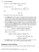
4.3 Express the function given in figure given below the
s-

t – domain and the

domain

This graph can be expressed as
= {u(t − 1) − u(t − 5)} + { (t − 2)u(t − 2) − (t − 3)u (t − 3)} + {u(t − 5) − (t − 5)u (t − 5) + (t − 6)u (t − 6)}
f (t ) = u (t − 1) + (t − 2)u(t − 2) − (t − 2)u(t − 3) − (t − 5)u(t − 5) + (t − 6)u(t − 6)

f ( s ) = L{ f (t )} =

e − s e −2 s e −3s e −3s
e −5 s e −6 s
+ 2 − 2 −
− 2 + 2
s

s
s
s
s
s
=

e − s − e −3s e −2 s + e −6 s − e −3s − e −5 s
+
s
s2


4.4 Sketch the following functions:
f (t ) = u (t ) − 2u(t − 1) + u(t − 3)

f (t ) = 3tu(t ) − 3u(t − 1) + u(t − 2)


4.5 The function f(t) has the Laplace transform

f ( S ) = (1 − 2e − s + e −2 s ) / s 2
obtain the function f(t) and graph f(t)
1 − 2 e − s + e −2 s
f ( s) =
s2

=

1 − e − s e − s − e −2 s

−
s2
s2

f (t ) = L−1{ f ( s )} = − (t − 1)u(t − 1) + tu(t ) − {(t − 1)u (t − 1) − (t − 2)u(t − 2)]
= tu(t ) − 2(t − 1)u (t − 1) + (t − 2)u(t − 2)
4.6 Determine f(t) at t = 1.5 and at t = 3 for following function:
f (t ) = 0.5u(t ) − 0.5u(t − 1) + (t − 3)u (t − 2)


At t = 1.5
f (t ) = 0.5u(t ) − 0.5u (t − 1) + (t − 3)u (t − 2)
f (1.5) = 0.5u(t ) − 0.5u(t − 1)
f (1.5) = 0.5 − 0.5 = 0

At t = 3

f (3) = 0.5 − 0.5 + (3 − 3) = 0

RESPONSE OF A FIRST ORDER SYSTEMS
5.1 A thermometer having a time constant of 0.2 min is placed in a
temperature bath and after the thermometer comes to equilibrium with
the bath, the temperature of the bath is increased linearly with time at the
rate of I deg C / min what is the difference between
the indicated
temperature and bath temperature
(a) 0.1 min
(b) 10. min
after the change in temperature begins.
© what is the maximum deviation between the indicated temperaturew

and bath temperature and when does it occurs.
(d) plot the forcing function and the response on the same graph. After the
long enough time buy how many minutes does the response lag the input.

Consider thermometer to be in equilibrium with
temperature Xs
X (t ) = X S + (1° / m )t , t > 0
as it is given that the temperture varies linearly
X(t)-Xs = t
Let X(t) = X(t) - Xs = t

temperature

bath at


Y(s) = G(s).X(s)
Y ( s) =

1 1
A
B C
=
+ + 2
2
1 + τs s 1 + τs s s

A = τ 2 B = − τ C =1

τ2

τ 1
Y ( s) =
− + 2
1 + τs s s
Y ( t ) = τe − t / τ − τ + t
(a) the difference between the indicated temperature and bath temperature
at t = 0.1 min = X(0.1)_ Y(0.1)
= 0.1 - (0.2e-0.1/0.2 - 0.2+0.1) since T = 0.2 given
= 0.0787 deg C
(b) t = 1.0 min
X(1) - Y(1) = 1- (0.2e-1/0.2 - 0.2 +1) = 0.1986
(c) Deviation D = -Y(t) +X(t)
= -τe-t/T+T =τ (-e-t/T+1)
For maximum value dD/dT = τ (-e-t/T+(_-1/T) = 0
-e-t/ = 0
as t tend to infinitive
D = τ (-e-t/T+(_-1/T) = τ =0.2 deg C

5.2 A mercury thermometer bulb in ½ in . long by 1/8 in diameter. The
glass envelope is very thin. Calculate the time constant in water flowing
at 10 ft / sec at a temperature of 100 deg F. In your solution , give a
summary which includes
(a) Assumptions used.
(b) Source of data
(c) Results


T = mCp/hA =

( ρAL)C p

h ( A + πDL)

Calculation of

NU d =

Re d =

Pr =

hD
= CRem (Pr) n
K

Dvρ

µ

Cpµ
K

=

(1 / 8 * 2.54 * 10 −2 )(10 * 0.3048)103
= 9677.4
10 −3

= 4.2 KJ / KgK

Source data: Recently, Z hukauskas has given c,m ,ξ,n values.

For Re = 967704
C = 0.26 & m = 0.6
NuD = hD/K = 0.193 (9677.4)*(6.774X10-3) = 130
.h = 25380

5.3 Given a system with the transfer function Y(s)/X(s) = (T1s+1)/(T2s+1).
Find Y(t) if X(t) is a unit step function. If T1/T2 = s. Sktech Y(t) Versus
t/T2. Show the numerical values of minimum, maximum and ultimate values
that may occur during the transient. Check these using the initial value
and final value theorems of chapter 4.

Y ( s) =

T1s + 1
T2 s + 1

X(s) =unit step function = 1 X(s) = 1/s


Y ( s) =

T1 s + 1
A
B
= +
s (T2 s + 1)
s iT2 s

A = 1 B = T1 - T2
Y ( s) =

1 T1 − T2
+
s 1 + T2 s

Y (t ) = 1 +

T1 − T2 −t / T2
e
T2

If T1/T2 = s then
Y (t ) = 1 + 4e − t / T2
Let t/T2 = x then Y (t ) = 1 + 4e

−x

Using the initial value theorem and final value theorem
Lim Y (T ) = Lim sY ( s )
S →∞

T →0

1
T s +1
s = T1 = 5
Lim 1
= Lim
S →∞ T s + 1
S →∞

1
T2
2
T2 +
s
T1 +

=

Lim Y (T ) = Lim sY ( s ) = Lim
T →0

Figure:

S →∞

S →0

T1 s + 1
=1
T2 s + 1