Fluid power system dynamicss
Bạn đang xem bản rút gọn của tài liệu. Xem và tải ngay bản đầy đủ của tài liệu tại đây (5.02 MB, 54 trang )
Fluid Power System Dynamics
William Durfee, Zongxuan Sun
and James Van de Ven
Department of Mechanical Engineering
University of Minnesota
A National Science Foundation
Engineering Research Center
FLUID POWER SYSTEM DYNAMICS
Center for Compact and Efficient Fluid Power
University of Minnesota
Minneapolis, USA
This book is available as a free, full-color PDF download from
sites.google.com/site/fluidpoweropencourseware/. The printed,
bound version can be purchased at cost on lulu.com.
Copyright and Distribution
Copyright is retained by the authors. Anyone may freely copy and
distribute this material for educational purposes, but may not sell the
material for profit. For questions about this book contact Will Durfee,
University of Minnesota,
c 2015
Version: September 25, 2015
Contents
Preface
1
1. Introduction
2
1.1. Overview . . . . . . . . . . . . . . . . . . . . . . . . . . . .
1.2. Fluid Power Examples . . . . . . . . . . . . . . . . . . . .
1.3. Analyzing Fluid Power Systems . . . . . . . . . . . . . .
2. Basic Principles of Fluid Power
10
2.1.
2.2.
2.3.
2.4.
Pressure and Flow . . . . . . . . . .
Power and Efficiency . . . . . . . .
Hydraulic Fluids . . . . . . . . . .
Fluid Behavior . . . . . . . . . . . .
2.4.1. Viscosity . . . . . . . . . . .
2.4.2. Bulk Modulus . . . . . . . .
2.4.3. Pascal’s Law . . . . . . . . .
2.4.4. High Forces . . . . . . . . .
2.5. Conduit Flow . . . . . . . . . . . .
2.5.1. Pressure Losses in Conduits
2.6. Bends and Fittings . . . . . . . . .
2.7. Orifice Flow . . . . . . . . . . . . .
.
.
.
.
.
.
.
.
.
.
.
.
.
.
.
.
.
.
.
.
.
.
.
.
.
.
.
.
.
.
.
.
.
.
.
.
.
.
.
.
.
.
.
.
.
.
.
.
.
.
.
.
.
.
.
.
.
.
.
.
.
.
.
.
.
.
.
.
.
.
.
.
.
.
.
.
.
.
.
.
.
.
.
.
.
.
.
.
.
.
.
.
.
.
.
.
.
.
.
.
.
.
.
.
.
.
.
.
.
.
.
.
.
.
.
.
.
.
.
.
.
.
.
.
.
.
.
.
.
.
.
.
.
.
.
.
.
.
.
.
.
.
.
.
.
.
.
.
.
.
.
.
.
.
.
.
.
.
.
.
.
.
.
.
.
.
.
.
.
.
.
.
.
.
.
.
.
.
.
.
.
.
.
.
.
.
.
.
.
.
.
.
.
.
.
.
.
.
.
.
.
.
.
.
.
.
.
.
.
.
.
.
.
.
.
.
.
.
.
.
.
.
.
.
.
.
.
.
.
.
.
.
.
.
.
.
.
.
.
.
.
.
.
.
.
.
.
.
.
.
.
.
.
.
.
.
.
.
.
.
.
.
.
.
.
.
.
.
.
.
.
.
.
.
.
.
.
.
.
.
.
.
.
.
.
.
.
.
.
.
.
.
.
.
.
.
.
.
.
.
.
.
.
.
.
.
.
.
.
.
.
.
.
.
.
.
.
.
.
.
.
.
.
.
.
.
.
.
.
.
.
.
.
.
.
.
.
.
3. Fluid Power Components
4. Hydraulic Circuit Analysis
Fluid Resistance . . . . . . .
Fluid Capacitance . . . . . .
Fluid Inertance . . . . . . .
Connection Laws and States
4.4.1. Connections . . . . .
10
12
13
14
14
15
17
18
20
22
25
27
29
3.1. Cylinders . . . . . . . . . . . . . . .
3.2. Pumps and Motors . . . . . . . . .
3.3. Control Valves . . . . . . . . . . . .
3.3.1. Dynamic Models for Valves
3.3.2. Valve Symbols . . . . . . . .
3.4. Accumulators . . . . . . . . . . . .
3.5. Filters . . . . . . . . . . . . . . . . .
3.6. Reservoirs . . . . . . . . . . . . . .
3.7. Hoses and Fittings . . . . . . . . .
4.1.
4.2.
4.3.
4.4.
2
3
7
29
32
34
35
36
37
38
39
40
41
.
.
.
.
.
.
.
.
.
.
.
.
.
.
.
.
.
.
.
.
42
43
45
45
45
iii
iv
Contents
4.4.2. State Variables . . . . . . . . . . . . . . . . . . . . .
4.5. Example Systems . . . . . . . . . . . . . . . . . . . . . . .
45
45
5. Bibliography
49
A. Fluid Power Symbols
50
Preface
This book was created because system dynamics courses in the standard mechanical engineering curriculum do not cover fluid power, even
though fluid power is essential to mechanical engineering and students
entering the work force are likely to encounter fluid power systems in
their job. Most system dynamics textbooks have a chapter or part of a
chapter on fluid power but typically the chapter is thin and does not
cover practical fluid power as is used in industry today. For example,
many textbooks confine their discussion of fluid power to liquid tank
systems and never even mention hydraulic cylinders, the workhorse of
today’s practical fluid power.
The material is intended for use in an introductory system dynamics
course that would teach analysis of mechanical translational, mechanical rotary and electrical system using differential equations, transfer
functions and time and frequency response. The material should be introduced toward the end of the course after the other domains and most
of the analysis methods have been covered. It replaces or supplements
any coverage of fluid power in the course textbook. The instruction can
pick and choose which sections will be covered in class or read by the
student. At the University of Minnesota, the material is used in course
ME 3281, System Dynamics and Control and in ME 4232, Fluid Power
Control Lab.
The book is a result of the Center for Compact and Efficient Fluid
Power (CCEFP) (www.ccefp.org), a National Science Foundation Engineering Research Center founded in 2006. CCEFP conducts basic and
applied research in fluid power with three thrust areas: efficiency, compactness, and usability. CCEFP has over 50 industrial affiliates and its
research is ultimately intended to be used in next generation fluid power
products. To ensure the material in the book is current and relevant, it
was reviewed by industry representatives and academics affiliated with
CCEFP.
Will Durfee
Zongxuan Sun
Jim Van de Ven
1
1. Introduction
1.1. Overview
Fluid power is the transmission of forces and motions using a confined,
pressurized fluid. In hydraulic fluid power systems the fluid is oil, or
less commonly water, while in pneumatic fluid power systems the fluid
is air.
Fluid power is ideal for high speed, high force, high power applications. Compared to all other actuation technologies, including electric
motors, fluid power is unsurpassed for force and power density and is
capable of generating extremely high forces with relatively lightweight
cylinder actuators. Fluid power systems have a higher bandwidth than
electric motors and can be used in applications that require fast starts,
stops and reversals, or that require high frequency oscillations. Because
oil has a high bulk modulus, hydraulic systems can be finely controlled
for precision motion applications. 1 Another major advantage of fluid
power is compactness and flexibility. Fluid power cylinders are relatively small and light for their weight and flexible hoses allows power
to be snaked around corners, over joints and through tubes leading to
compact packaging without sacrificing high force and high power. A
good example of this compact packaging are Jaws of Life rescue tools
for ripping open automobile bodies to extract those trapped within.
Fluid power is not all good news. Hydraulic systems can leak oil at
connections and seals. Hydraulic power is not as easy to generate as
electric power and requires a heavy, noisy pump. Hydraulic fluids can
cavitate and retain air resulting in spongy performance and loss of precision. Hydraulic and pneumatic systems become contaminated with particles and require careful filtering. The physics of fluid power is more
complex than that of electric motors which makes modeling and control more challenging. University and industry researchers are working
hard not only to overcome these challenges but also to open fluid power
to new applications, for example tiny robots and wearable power-assist
tools.
1 While conventional thinking was that pneumatics were not useful for precision control, recent advances in pneumatic components and pneumatic control theory has opened
up new opportunities for pneumatics in precision control.
2
1.2. Fluid Power Examples
3
Figure 1.1.: Caterpillar 797B mining truck. Source: Caterpillar
1.2. Fluid Power Examples
Fluid power is pervasive, from the gas spring that holds you up in the
office chair you are sitting on, to the air drill used by dentists, to the
brakes in your car, to practically every large agriculture, construction
and mining machine including harvesters, drills and excavators.
The Caterpillar 797B mining truck is the largest truck in the world at
3550 hp (Fig. 1.1). It carries 400 tons at 40 mph, uses 900 g of diesel per
12 hr shift, costs about $6M and has tires that are about $60,000 each.
It is used in large mining operations such as the Hull-Rust-Mahoning
Open Pit Iron Mine, the world’s largest open pit iron mine, located in
Hibbing MN and the Muskeg River Mine in Alberta Canada.2 The 797B
uses fluid power for many of its internal actuation systems, including
lifting the fully loaded bed.
Shultz Steel, an aerospace company in South Gate CA, has a 40,000ton forging press that weighs over 5.2 million pounds (Fig. 1.2). It is
the largest press in the world and is powered by hydraulics operating at
6,600 psi requiring 24 700 hp pumps.
The Multi-Axial Subassemblage Testing (MAST) Laboratory is located
at the University of Minnesota and is used to conduct three-dimensional,
quasi-static testing of large scale civil engineering structures, including
2 ”New Tech to Tap North America’s Vast Oil Reserves”, Popular Mechanics, March
2007.
4
1. Introduction
Figure 1.2.: 40,000 ton forging press. Source: Shultz Steel.
buildings, to determine behavior during earthquakes (Fig. 1.3). The
MAST system, constructed by MTS Systems, has eight hydraulic actuators that can each push or pull with a force of 3910 kN.
The Caterpillar 345C L excavator is used in the construction industry
for large digging and lifting operations and has a 345 hp engine (Fig.
1.4). The 345C L operates at a hydraulic pressure of 5,511 psi to generate
a bucket digging force of 60,200 lbs and a lift force of up to 47,350 lbs.
A feller buncher is a large forestry machine that cuts trees in place
(Fig. 1.5).
Some of the fastest roller coasters in the world get their initial launch
from hydraulics and pneumatics. (Fig. 1.6). Hydraulic launch assist systems pump hydraulic fluid into a bank of accumulators storing energy
as a compressed gas. At launch, the energy is suddenly released into a
hydraulic motor whose output shaft drives a cable drum with the cable
rapidly bringing the train from rest to very high velocities. The Kingda
Ka at Six Flags Great Adventure uses this launch and reaches 128 mph
in 3.5 s. The Hypersonic SLC at Kings Dominion ups the ante with a
compressed air launch system that accelerates riders to 81 mph in 1.8 s.
Most automatic transmissions have hydraulically actuated clutches
and bands to control the gear ratios. Fluid is routed through internal
passageways in the transmission case rather than through hoses (Fig.
1.7)
The dental drill is used to remove small volumes of decayed tooth
1.2. Fluid Power Examples
5
Figure 1.3.: MAST Laboratory for earthquake simulation. Source: MAST Lab.
Figure 1.4.: Caterpillar 345C L excavator. Source: Caterpillar.
6
1. Introduction
Figure 1.5.: Feller buncher. Souce: Wikipedia image.
Figure 1.6.: Hypersonic XLC roller coaster with hydraulic lanuch assist. Source:
Wikipedia image.
1.3. Analyzing Fluid Power Systems
7
Figure 1.7.: Mercedes-Benz automatic transmission model.
prior to inserting a filling (Fig. 1.8). Modern drills rotate at up to 500,000
rpm using an air turbine and use a burr bit for cutting. The hand piece
can cost up to $800. Pneumatic drills are used because they are smaller,
lighter and faster than electric motor drills. The compressor is located
away from the drill and pressurized air is piped to the actuator.
Hydraulic microdrives are used during surgery to position recording
electrodes in the brain with micron accuracy (Fig. 1.9). Master and slave
cylinders have a 1:1 ratio and are separated by three to four feet of fluid
filled cable.
1.3. Analyzing Fluid Power Systems
Analyzing the system dynamics of fluid power means using differential equations and simulations to examine the pressures and flows in
components of a fluid power circuit, and the forces and motions of the
mechanisms driven by the fluid power. For example, in an excavator,
the engineer would be interested in determining the diameter and stroke
length of the cylinder that is required to drive the excavator bucket and
how the force and velocity of the bucket changes with time as the valves
Figure 1.8.: A dental handpiece. Source: Wikipedia image.
8
1. Introduction
Figure 1.9.: Hydraulic microdrive for neural recording electrode placement.
Source: Stoelting Co.
to the cylinder are actuated. Because fluid power systems change with
time and because fluid power systems have energy storage elements,
a dynamic system analysis approach must be taken which means the
use of linear and nonlinear differential equations, linear and nonlinear
simulations, time responses, transfer functions and frequency analysis.
Fluid power is one domain within the field of system dynamics, just
as mechanical translational, mechanical rotational and electronic networks are system dynamic domains. Fluid power systems can be analyzed with the same mathematical tools used to describe spring-massdamper or inductor-capacitor-resistor systems. Like the other domains,
fluid power has fundamental power variables and system elements connected in networks. Unlike other domains many fluid power elements
are nonlinear which makes closed-form analysis somewhat more challenging, but not difficult to simulate. Many concepts from transfer functions and basic closed loop control systems are used to analyze fluid
power circuits, for example the response of a servovalve used for precision control of hydraulic pistons. 3
Like all system dynamics domains, fluid power is characterized by
two power variables that when multiplied form power, and ideal lumped
elements including two energy storing elements, one energy dissipating
element, a flow source element and a pressure source element. Table
1.1 shows the analogies between fluid power elements and elements in
other domains. Lumping fluid power systems into elements is useful
3 See ”‘Transfer Functions for Mood Servovalves”’ available on-line in the technical
documents section of the Moog company web site.
1.3. Analyzing Fluid Power Systems
9
Table 1.1.: Element analogies in several domains.
Domain
Power
Variable 1
Power
Variable 2
Storage
Element 1
Storage
Element 2
Dissipative
Element
Translational
Rotational
Electrical
Fluid Power
Force, F
Torque, T
Current, I
Flow, Q
Velocity, V
Velocity, ω
Voltage, V
Pressure, P
Mass, M
Inertia, J
Inductor, L
Inertance, If
Spring, K
Spring, K
Capacitor, C
Capacitor, Cf
Damper, B
Damper, B
Resistor, R
Resistance, Rf
when analyzing complex circuits.
2. Basic Principles of Fluid Power
2.1. Pressure and Flow
Fluid power is characterized by two main variables, pressure and flow,
whose product is power. Pressure P is force per unit area and flow Q
is volume per time. Because pneumatics uses compressible gas as the
fluid, mass flow rate Qm is used for the flow variable when analyzing
pneumatic systems. For hydraulics, the fluid is generally treated as incompressible, which means ordinary volume flow Q can be used.
Pressure is reported several common units that include pounds per
square inch (common engineering unit in the U.S.), pascal (one newton
per square meter, the SI unit), megapascal and bar. Table 2.1 shows how
pressure units are related. For engineering, it is best to do calculations
and simulations in SI units, but to report in SI and the conventional
engineering unit.
Pressure is an across type variable, which means that it is always measured with respect to a reference just like voltage in an electrical system.
As shown in Figure 2.1, one can talk about the pressure across a fluid
power element such as a pump or a valve, which is the pressure differential from one side to the other, but when describing the pressure
at a point, for example the pressure of fluid at one point in a hose, it is
always with respect to a reference pressure. Reporting absolute pressure
means that the pressure is measured with respect to a perfect vacuum.
It is more common to measure and report gauge pressure, the pressure
relative to ambient atmospheric pressure (0.10132 mPA, 14.7 psi at sea
level). The distinction is critical when analyzing the dynamics of pneumatic systems because the ideal gas law that models the behavior of air
is based on absolute pressure.
Table 2.1.: Conversions between pressure units
1 Pa
1 Mpa
1 bar
1 psi
10
pascal
(Pa)
megapascal
(Mpa)
bar
(bar)
lbs-sq-in
(psi)
1
106
105
6895
10−6
1
0.1
6.895 × 10⁻³
10−5
10
1
0.06895
145.04 × 10⁻⁶
145
14.5
1
2.1. Pressure and Flow
11
Figure 2.1.: Pressure is measured with respect to a reference.
Pressure is measured with a mechanical dial type pressure gage or
with an electronic pressure transducer that outputs a voltage proportional to pressure (Fig. 2.2). Almost all pressure transducers report
gauge pressure because they expose their reference surface to atmosphere.
Volume flow rate is reported in gallons per minute, liters per minute
and cubic meters per second (SI unit). Table 2.2 shows how flow rate
units are related.
Flow is a through type variable, which means it is volume of fluid flowing through an imaginary plane at one location. Like current in an electrical system, there is no reference point. Flow is measured with a flow
meter placed in-line with the fluid circuit. One common type of flow
meter contains a turbine, vane or paddle wheel that spins with the flow.
Another type has a narrowed passage or an orifice and flow is estimated
by measuring the differential pressure across the obstruction. A Pitot
tube estimates velocity by measuring the dynamic pressure, which is
the difference between the stagnation pressure and static pressure. Figure 2.3 shows some common types of flow meters. Because flow meters
restrict the flow, they are used sparingly in systems where small pressure drops matter.
Figure 2.2.: Dial pressure gauge and electronic pressure transducer.
12
2. Basic Principles of Fluid Power
Table 2.2.: Conversions between volume flow rate units
1 gpm
1 lpm
1 m3 /s
gallon/minute
(gpm)
liter/minute
(lpm)
cubicmeter/second
(m3 /s)
1
0.264
1.585 × 10⁴
3.785
1
6 × 10⁴
6.31 × 10⁻⁵
1.67 × 10⁻⁵
1
2.2. Power and Efficiency
The power available at any one point in a fluid power system is the
pressure times the flow at that point
power = P × Q
(2.1)
For the power available in a conduit, the pressure in Equation 2.1 is
the pressure relative to the pressure in the system reservoir, which is
typically at atmospheric pressure.
Example 2.2.1. The hose supplying the cylinder operating the bucket of
a large excavator has fluid at 1000 psi flowing at 5 gpm. What is the
available power in the line?
Figure 2.3.: Types of flowmeters. Top row: turbine, digital paddle, variable area.
Bottom row is a dual-rotor turbine flowmeter with a cutaway.
2.3. Hydraulic Fluids
13
Solution: For most engineering examples, the reported pressure is a
gage pressure, which means the hose is operating at 1000 psi above atmospheric pressure, the pressure of the reservoir. To calculate the power
1000 psi × 6895 Pa/psi = 6.9×10⁶ Pa
5 gpm × 6.31×10−5 m3 /s/gpm = 31.6×10⁻⁵ m3 /s
Power = 6.9 × 106 × 31.6 × 10−5 = 2180 watts = 2.9 horsepower
Components such as cylinders, motors and pumps have input and
output powers, which can be used to calculate the efficiency of the component. For example, pressured fluid flows into a cylinder and the cylinder extends. The input power is the pressure of the fluid times its flow
rate while the output power is the compression force in the cylinder
rod times the rod extension velocity. Dividing output power by input
power yields the efficiency of the component. The same can be done for
components such as an orifice. The efficiency of the orifice is the output
pressure divided by the input pressure because the flow rate is the same
on either side of the orifice.
2.3. Hydraulic Fluids
The main purpose of the fluid in a fluid power system is to transmit
power. There are other, practical considerations that dictate the specific
fluids used in real hydraulic systems. The fluids must cool the system
by dissipation of heat in a radiator or reservoir, must help with sealing
to prevent leaks, must lubricate sliding and rotating surfaces such as
those in motors and cylinders, must not corrode components and must
have a long life without chemical breakdown.
The earliest hydraulic systems used water for the fluid. While water is safe for humans and environment, cheap and readily available,
it has significant disadvantages for hydraulic applications. Water provides almost no lubrication, has low viscosity and leaks by seals, easily
cavitates when subjected to negative pressures, has a narrow temperature range between freezing and boiling (0 to 100 ◦ C), is corrosive to the
steels used extensively in hydraulic components and is a friendly environment for bacteria and algae growth, which is why swimming pools
are chlorinated.
Modern hydraulic system use petroleum based oils, with additives
to inhibit foaming and corrosion. Petroleum oils are inexpensive, provide good lubricity and, with additives, have long life. The brake and
automatic transmission fluids in your car are examples.
14
2. Basic Principles of Fluid Power
Figure 2.4.: Viscosity related hydraulic system losses.
2.4. Fluid Behavior
2.4.1. Viscosity
All fluids, including oil and air have fundamental properties and follow basic fluid mechanics laws. The viscosity of a fluid is its resistance
to flow. Some fluids, like water, are thin and have low viscosity while
others like honey are thick and have high viscosity. The fluids for hydraulic systems are a compromise. If the viscosity is too low, fluid will
leak by internal seals causing a volumetric loss of efficiency. If the viscosity is too high, the fluid is difficult to push through hoses, fittings
and valves causing a loss of mechanical efficiency. Figure 2.4 shows this
tradeoff and indicates that a medium viscosity fluid is best for hydraulic
applications.
The dynamic viscosity (also known as the absolute viscosity) is the
shearing resistance of the fluid and is measured by placing the fluid
between two plates and shearing one plate with respect to the other.
The symbol for dynamic viscosity is the Greek letter mu (µ). The SI unit
for dynamic viscosity is the pascal-second (Pa-s), but the more common
unit is the centipoise (cP), with 1 cP = 0.001 Pa-s. The dynamic viscosity
of water at 20 ◦ C is 1.00 cP
It is easier to measure and more common to report the kinematic viscosity of a fluid, the ratio of the viscous forces to inertial forces. The symbol
for kinematic viscosity is the Greek letter nu (ν). Kinematic viscosity
can be measured by the time it takes a volume of oil to flow through a
capillary. The SI unit for kinematic viscosity is m2 /s but the more com-
2.4. Fluid Behavior
15
Figure 2.5.: The viscosity of hydraulic oils varies with temperature.
mon unit is the centistoke (cSt) which is 1 mm2 /s. The conversion is
1m2 /s = 106 cSt = 104 stokes
If ρ is the fluid density, the kinematic and dynamic viscosity are related by
µ
ν=
(2.2)
ρ
The kinematic viscosity of water over a wide range of temperature is 1
cSt while common hydraulic oils at 40 ◦ C are in the range of 20-70 cSt.
Sometimes hydraulic oil kinematic viscosity is expressed in Saybolt Universal Seconds (SUS), which comes from the oil properties being measured on a Saybolt viscometer.
Viscosity changes with temperature; as fluid warms up it flows more
easily. One reason your car is hard to start on a very cold morning is
that the engine oil thickened overnight in the cold. The viscosity index
VI expresses how much viscosity changes with temperature. Fluids with
a high VI are desirable because they experience less change in viscosity
with temperature. Figure 2.5 shows how viscostiy changes for typical
hydraulic fluids.
2.4.2. Bulk Modulus
In many engineering applications, liquids are assumed to be completely
incompressible even though all materials can be compressed to some
16
2. Basic Principles of Fluid Power
Figure 2.6.: Fluid bulk modulous. Liquids are nearly incompressible (left), ex-
cept when there is trapped air, as shown on the right.
degree. In some hydraulic applications, the tiny compressibility of oil
turns out to be important because the pressures are high, up to 5,000 psi.
The bulk modulus of the fluid is the property that indicates the springiness of the fluid and is defined as the pressure needed to cause a given
decrease in volume. A typical oil will decrease about 0.5% in volume for
every 1000 psi increase in pressure. When the compressibility is significant, it is modeled as a fluid capacitor (spring) and often is lumped in
with the fluid capacitance of the accumulator (see Section 3.4).
When air bubbles are entrained in the hydraulic oil, the bulk modulus
drops and the fluid becomes springy (Fig. 2.6). You may have experienced this when the brake pedal in your car felt spongy. The solution
was to bleed the brake system, which releases the trapped air so that the
brake fluid becomes stiff again.
Another way that the fluid can change properties is if the pressure fall
below the vapor pressure of the liquid causing the formation of vapor
bubbles. When the bubbles collapse, a shock wave is produced that can
erode nearby surfaces. Cavitation damage can be a problem for propellers and for fluid power pumps with the erosion greatly shortening
the lifetime of components.
The bulk modulus β is defined as
β=
∆P
∆V /V
(2.3)
where V is the original volume of liquid and ∆V is the change in volume
of the liquid when subjected to a pressure change of ∆P . Because ∆V /V
is dimensionless, the units of β are pressure. Water has a bulk modulus
of 3.12 × 10⁵ psi (2.15 GPa) while hydraulic oils have a bulk modulus
between 2 × 10⁵ and 3 × 10⁵ psi (SAE 30 oil is 2.2 × 10⁵ psi = 1.5 GPa),
2.4. Fluid Behavior
17
but can drop way down if air is entrained.
Example 2.4.1. A piston pushes down on a volume of SAE 30 oil trapped
in a cylinder like the one shown in Figure 2.6. The cylinder bore is 5 in.
and the height of the unstressed column of oil is 4 in. The oil has a bulk
modulus β = 2.2 × 10⁵ psi. When a force of 10,000 lbs is applied to the
piston, how much does the piston displace?
Solution: Use Equation 2.3 to calculate the change in volume
∆P V
(F/A)(Ah)
Fh
=
=
β
β
β
4
(1 × 10 ) × 4
=
2.2 × 105
= .18 cu. in.
∆V =
The change in height is
∆V
A
.18
=
π(5/2)2
= 0.0092 in.
∆h =
2.4.3. Pascal’s Law
Pascal’s Law states that in a confined fluid at rest, pressure acts equally
in all directions and acts perpendicular to the confining walls (Fig. 2.7).
This means that all chambers, hoses and spaces in a fluid power system
that have open passageways between them are at equal pressure so long
as the fluid is not moving.
Pascal’s Law makes it easy to understand the operation of a simple
hydraulic amplifier. Figure 2.8 shows how it works. The piston on the
right is 25 times the area of the piston on the left. Pushing down with
10 lbs on the left piston will lift a 250 lb load on the right because the
pressure of 10 psi is the same everywhere.
18
2. Basic Principles of Fluid Power
Figure 2.7.: Pascal’ Law. Fluid at rest has same pressure everywhere and acts at
right angles against the walls.
2.4.4. High Forces
The crowning glory of fluid power is the ability for small, light fluid
power cylinders to produce extremely large forces. Consider the Caterpillar 345D hydraulic excavator shown in Figure 2.9. The bore (diameter) of the cylinder that drives the stick is 7.5 in. and the maximum
working pressure is 5511 psi. The peak force in the cylinder is therefore
F = P × A = 5511 × π × (7.5/2)2 = 243, 468 lbs
or over 120 tons! It is impossible to produce this force using electric
motors.
Force can be increased two ways, raising the pressure or increasing
the bore of the cylinder. Force is proportional to pressure but goes as the
square of the bore, which means small increases in cylinder size results
Figure 2.8.: Hydraulic amplifier. Pushing down with 10 lbs on the left piston
raises the 250 lb. weight on the right piston.
2.4. Fluid Behavior
19
Figure 2.9.: A large excavator. Source: Caterpillar.
in large increases in force. For example, consider a small pneumatic
cylinder with a 7/16 in. bore running at 60 psi. This cylinder can push
with 9 lbs of force. But, as shown in Figure 2.10, force goes up as bore
squared and a 4 in. bore cylinder at the same 60 psi can push with 754
lbs of force.
Of course the extra force does not come free. A larger cylinder requires a greater volume of fluid to move the load than a smaller cylinder,
the practical result of the requirement that power be conserved.
Figure 2.10.: Force in a cylinder acting at 60 psi. goes up with the square of the
bore.
20
2. Basic Principles of Fluid Power
Figure 2.11.: Hoses on an excavator.
2.5. Conduit Flow
In electromechanical actuation systems, power is carried to motors through
appropriately sized, low-resistance wires with negligible power loss.
This is not the case for fluid power systems where the flow of oil through
hydraulic hoses and pipes can result in energy losses due to internal
fluid friction and the friction against the walls of the conduit (Fig. 2.11).
Designers size the diameter and length of hydraulic hoses to minimize
these losses. The other cause of major losses in fluid power systems is
the orifice drag of valves and fittings. These will be discussed in Section 3 These loses are modeled as nonlinear resistances in the hydraulic
circuit.
Conduit flow properties can be analyzed using basic principles of
fluid mechanics. Typical flow patterns through pipes are shown in Figure 2.12. At low velocities, the flow is smooth and uniform while at
higher velocities the flow turns turbulent. Turbulent flow can also be
caused by sudden changes in direction or when the area suddenly changes,
conditions that are common in hydraulic systems. Turbulent flow has
higher friction, which results in greater heat losses and lower operating
efficiencies. This is a practical concern for designers of hydraulic systems because every right angle fitting designed into the system lowers
the system efficiency.
The Reynolds number, the non-dimensional ratio of inertial to viscous
forces, is commonly used to characterize the flow in pipes
Re =
ρV Dh
V Dh
=
µ
ν
(2.4)
where ρ is the density (kg/m2 ), V is the mean fluid velocity (m/s), Dh is
the hydraulic diameter (m), µ is the dynamic viscosity (Pa-s) and ν is the
2.5. Conduit Flow
21
Figure 2.12.: Laminar and turbulent flow through a pipe.
kinematic viscosity. For circular conduits, the hydraulic diameter is the
same as the pipe diameter. The more general formula, which accounts
for non-circular pipes and hoses is
Dh =
4A
S
(2.5)
where A is the cross-sectional area of the conduit and S is the perimeter.
For a circle this formula reduces to diameter of the circle.
For fully developed pipe flow, if Re < 2100 the flow is laminar, if
2100 < Re < 4000 the flow is in transition, neither laminar or turbulent,
and if Re > 4000 the flow is turbulent. These are approximations as
the actual flow type will depend on local conditions and local geometry, which is why you may find other sources using different Reynolds
number break points to define the flow type.
Example 2.5.1. A hydraulic hose with internal diameter of 1.0 in. is
carrying oil with kinematic viscosity 50 cSt at a flow rate of 20 gpm.
Calculate the Reynolds number and determine if the flow is laminar or
turbulent.
Solution: Convert to SI units.
Q = 20 gpm = .00126 cu-m/s
D = 1.0 in. = .0254 m
ν = 50 cSt = 5.0 × 10⁻⁵ m2 /s
Find the average velocity
V =
4Q
(4)(.00126)
=
= 2.49 m/s
πD2
(3.142)(.0254)2
Calculate the Reynolds number
Re =
VD
(2.49)(.0254)
=
= 1265
ν
5.0 × 10⁻⁵