Introduction to python for economotric statistics and data analysis
Bạn đang xem bản rút gọn của tài liệu. Xem và tải ngay bản đầy đủ của tài liệu tại đây (2.54 MB, 405 trang )
Introduction to Python for Econometrics, Statistics and Data Analysis
Kevin Sheppard
University of Oxford
Tuesday 5th August, 2014
-
©2012, 2013, 2014 Kevin Sheppard
2
Changes since the Second Edition
Version 2.2.1 (August 2014)
• Fixed typos reported by a reader – thanks to Ilya Sorvachev
Version 2.2 (July 2014)
• Code verified against Anaconda 2.0.1.
• Added diagnostic tools and a simple method to use external code in the Cython section.
• Updated the Numba section to reflect recent changes.
• Fixed some typos in the chapter on Performance and Optimization.
• Added examples of joblib and IPython’s cluster to the chapter on running code in parallel
Version 2.1 (February 2014)
• New chapter introducing object oriented programming as a method to provide structure and organization to related code.
• Added seaborn to the recommended package list, and have included it be default in the graphics
chapter.
• Based on experience teaching Python to economics students, the recommended installation has
been simplified by removing the suggestion to use virtual environment. The discussion of virtual
environments as been moved to the appendix.
• Rewrote parts of the pandas chapter.
• Code verified against Anaconda 1.9.1.
Version 2.02 (November 2013)
• Changed the Anaconda install to use both create and install, which shows how to install additional
packages.
• Fixed some missing packages in the direct install.
• Changed the configuration of IPython to reflect best practices.
• Added subsection covering IPython profiles.
i
Version 2.01 (October 2013)
• Updated Anaconda to 1.8 and added some additional packages to the installation for Spyder.
• Small section about Spyder as a good starting IDE.
ii
Notes to the 2nd Edition
This edition includes the following changes from the first edition (March 2012):
• The preferred installation method is now Continuum Analytics’ Anaconda. Anaconda is a complete
scientific stack and is available for all major platforms.
• New chapter on pandas. pandas provides a simple but powerful tool to manage data and perform
basic analysis. It also greatly simplifies importing and exporting data.
• New chapter on advanced selection of elements from an array.
• Numba provides just-in-time compilation for numeric Python code which often produces large performance gains when pure NumPy solutions are not available (e.g. looping code).
• Dictionary, set and tuple comprehensions
• Numerous typos
• All code has been verified working against Anaconda 1.7.0.
iii
iv
Contents
1
2
3
4
Introduction
1
1.1
Background . . . . . . . . . . . . . . . . . . . . . . . . . . . . . . . . . . . . . . . . . . . . .
1
1.2
Conventions . . . . . . . . . . . . . . . . . . . . . . . . . . . . . . . . . . . . . . . . . . . . .
2
1.3
Important Components of the Python Scientific Stack . . . . . . . . . . . . . . . . . . . . . . . .
3
1.4
Setup
. . . . . . . . . . . . . . . . . . . . . . . . . . . . . . . . . . . . . . . . . . . . . . . .
4
1.5
Using Python
. . . . . . . . . . . . . . . . . . . . . . . . . . . . . . . . . . . . . . . . . . . .
6
1.6
Exercises
1.A
Frequently Encountered Problems . . . . . . . . . . . . . . . . . . . . . . . . . . . . . . . . . . 17
1.B
register_python.py . . . . . . . . . . . . . . . . . . . . . . . . . . . . . . . . . . . . . . . . . . 18
1.C
Advanced Setup . . . . . . . . . . . . . . . . . . . . . . . . . . . . . . . . . . . . . . . . . . . 19
. . . . . . . . . . . . . . . . . . . . . . . . . . . . . . . . . . . . . . . . . . . . . . 17
Python 2.7 vs. 3 (and the rest)
27
2.1
Python 2.7 vs. 3 . . . . . . . . . . . . . . . . . . . . . . . . . . . . . . . . . . . . . . . . . . . 27
2.2
Intel Math Kernel Library and AMD Core Math Library . . . . . . . . . . . . . . . . . . . . . . . . 27
2.3
Other Variants . . . . . . . . . . . . . . . . . . . . . . . . . . . . . . . . . . . . . . . . . . . . 28
2.A
Relevant Differences between Python 2.7 and 3 . . . . . . . . . . . . . . . . . . . . . . . . . . . 29
Built-in Data Types
31
3.1
Variable Names . . . . . . . . . . . . . . . . . . . . . . . . . . . . . . . . . . . . . . . . . . . 31
3.2
Core Native Data Types . . . . . . . . . . . . . . . . . . . . . . . . . . . . . . . . . . . . . . . 32
3.3
Python and Memory Management . . . . . . . . . . . . . . . . . . . . . . . . . . . . . . . . . . 42
3.4
Exercises
. . . . . . . . . . . . . . . . . . . . . . . . . . . . . . . . . . . . . . . . . . . . . . 44
Arrays and Matrices
47
4.1
Array . . . . . . . . . . . . . . . . . . . . . . . . . . . . . . . . . . . . . . . . . . . . . . . . . 47
4.2
Matrix . . . . . . . . . . . . . . . . . . . . . . . . . . . . . . . . . . . . . . . . . . . . . . . . 49
4.3
1-dimensional Arrays
. . . . . . . . . . . . . . . . . . . . . . . . . . . . . . . . . . . . . . . . 50
4.4
2-dimensional Arrays
. . . . . . . . . . . . . . . . . . . . . . . . . . . . . . . . . . . . . . . . 51
4.5
Multidimensional Arrays . . . . . . . . . . . . . . . . . . . . . . . . . . . . . . . . . . . . . . . 51
4.6
Concatenation . . . . . . . . . . . . . . . . . . . . . . . . . . . . . . . . . . . . . . . . . . . . 51
4.7
Accessing Elements of an Array . . . . . . . . . . . . . . . . . . . . . . . . . . . . . . . . . . . 52
4.8
Slicing and Memory Management . . . . . . . . . . . . . . . . . . . . . . . . . . . . . . . . . . 57
v
4.9
import and Modules . . . . . . . . . . . . . . . . . . . . . . . . . . . . . . . . . . . . . . . . 59
4.10 Calling Functions
4.11 Exercises
5
. . . . . . . . . . . . . . . . . . . . . . . . . . . . . . . . . . . . . . . . . . 59
. . . . . . . . . . . . . . . . . . . . . . . . . . . . . . . . . . . . . . . . . . . . . . 61
Basic Math
63
5.1
Operators . . . . . . . . . . . . . . . . . . . . . . . . . . . . . . . . . . . . . . . . . . . . . . 63
5.2
Broadcasting . . . . . . . . . . . . . . . . . . . . . . . . . . . . . . . . . . . . . . . . . . . . . 64
5.3
Array and Matrix Addition (+) and Subtraction (-) . . . . . . . . . . . . . . . . . . . . . . . . . . 65
5.4
Array Multiplication (*) . . . . . . . . . . . . . . . . . . . . . . . . . . . . . . . . . . . . . . . . 66
5.5
Matrix Multiplication (*) . . . . . . . . . . . . . . . . . . . . . . . . . . . . . . . . . . . . . . . 66
5.6
Array and Matrix Division (/) . . . . . . . . . . . . . . . . . . . . . . . . . . . . . . . . . . . . . 66
5.7
Array Exponentiation (**) . . . . . . . . . . . . . . . . . . . . . . . . . . . . . . . . . . . . . . . 66
5.8
Matrix Exponentiation (**) . . . . . . . . . . . . . . . . . . . . . . . . . . . . . . . . . . . . . . 67
5.9
Parentheses . . . . . . . . . . . . . . . . . . . . . . . . . . . . . . . . . . . . . . . . . . . . . 67
5.10 Transpose . . . . . . . . . . . . . . . . . . . . . . . . . . . . . . . . . . . . . . . . . . . . . . 67
5.11 Operator Precedence . . . . . . . . . . . . . . . . . . . . . . . . . . . . . . . . . . . . . . . . 67
5.12 Exercises
6
7
Basic Functions and Numerical Indexing
9
71
6.1
Generating Arrays and Matrices . . . . . . . . . . . . . . . . . . . . . . . . . . . . . . . . . . . 71
6.2
Rounding
6.3
Mathematics . . . . . . . . . . . . . . . . . . . . . . . . . . . . . . . . . . . . . . . . . . . . . 75
6.4
Complex Values . . . . . . . . . . . . . . . . . . . . . . . . . . . . . . . . . . . . . . . . . . . 77
6.5
Set Functions . . . . . . . . . . . . . . . . . . . . . . . . . . . . . . . . . . . . . . . . . . . . 77
6.6
Sorting and Extreme Values . . . . . . . . . . . . . . . . . . . . . . . . . . . . . . . . . . . . . 78
6.7
Nan Functions . . . . . . . . . . . . . . . . . . . . . . . . . . . . . . . . . . . . . . . . . . . . 80
6.8
Functions and Methods/Properties
6.9
Exercises
. . . . . . . . . . . . . . . . . . . . . . . . . . . . . . . . . . . . . . . . . . . . . . 82
Special Arrays
83
7.1
8
. . . . . . . . . . . . . . . . . . . . . . . . . . . . . . . . . . . . . . . . . . . . . . 68
Exercises
. . . . . . . . . . . . . . . . . . . . . . . . . . . . . . . . . . . . . . . . . . . . . . 74
. . . . . . . . . . . . . . . . . . . . . . . . . . . . . . . . . 81
. . . . . . . . . . . . . . . . . . . . . . . . . . . . . . . . . . . . . . . . . . . . . . 84
Array and Matrix Functions
85
. . . . . . . . . . . . . . . . . . . . . . . . . . . . . . . . . . . . . . . . . . . . . . . . 85
8.1
Views
8.2
Shape Information and Transformation
8.3
Linear Algebra Functions
8.4
Exercises
. . . . . . . . . . . . . . . . . . . . . . . . . . . . . . . 86
. . . . . . . . . . . . . . . . . . . . . . . . . . . . . . . . . . . . . . 93
. . . . . . . . . . . . . . . . . . . . . . . . . . . . . . . . . . . . . . . . . . . . . . 96
Importing and Exporting Data
99
. . . . . . . . . . . . . . . . . . . . . . . . . . . . . . . . . . . . 99
9.1
Importing Data using pandas
9.2
Importing Data without pandas
9.3
Saving or Exporting Data using pandas . . . . . . . . . . . . . . . . . . . . . . . . . . . . . . . 106
. . . . . . . . . . . . . . . . . . . . . . . . . . . . . . . . . . . 100
vi
9.4
Saving or Exporting Data without pandas . . . . . . . . . . . . . . . . . . . . . . . . . . . . . . 106
9.5
Exercises
. . . . . . . . . . . . . . . . . . . . . . . . . . . . . . . . . . . . . . . . . . . . . . 107
10 Inf, NaN and Numeric Limits
109
10.1 inf and NaN . . . . . . . . . . . . . . . . . . . . . . . . . . . . . . . . . . . . . . . . . . . . . 109
10.2 Floating point precision
10.3 Exercises
. . . . . . . . . . . . . . . . . . . . . . . . . . . . . . . . . . . . . . . 109
. . . . . . . . . . . . . . . . . . . . . . . . . . . . . . . . . . . . . . . . . . . . . . 110
11 Logical Operators and Find
113
11.1 >, >=, <, <=, ==, != . . . . . . . . . . . . . . . . . . . . . . . . . . . . . . . . . . . . . . . . . 113
11.2 and, or, not and xor . . . . . . . . . . . . . . . . . . . . . . . . . . . . . . . . . . . . . . . . . 114
11.3 Multiple tests . . . . . . . . . . . . . . . . . . . . . . . . . . . . . . . . . . . . . . . . . . . . . 115
11.4 is* . . . . . . . . . . . . . . . . . . . . . . . . . . . . . . . . . . . . . . . . . . . . . . . . . 116
11.5 Exercises . . . . . . . . . . . . . . . . . . . . . . . . . . . . . . . . . . . . . . . . . . . . . . 117
12 Advanced Selection and Assignment
12.1 Numerical Indexing
119
. . . . . . . . . . . . . . . . . . . . . . . . . . . . . . . . . . . . . . . . . 119
12.2 Logical Indexing . . . . . . . . . . . . . . . . . . . . . . . . . . . . . . . . . . . . . . . . . . . 124
12.3 Performance Considerations and Memory Management . . . . . . . . . . . . . . . . . . . . . . . 128
12.4 Assignment with Broadcasting . . . . . . . . . . . . . . . . . . . . . . . . . . . . . . . . . . . . 128
12.5 Exercises
. . . . . . . . . . . . . . . . . . . . . . . . . . . . . . . . . . . . . . . . . . . . . . 130
13 Flow Control, Loops and Exception Handling
133
13.1 Whitespace and Flow Control . . . . . . . . . . . . . . . . . . . . . . . . . . . . . . . . . . . . 133
13.2 if . . . elif . . . else . . . . . . . . . . . . . . . . . . . . . . . . . . . . . . . . . . . . . . . . 133
13.3 for
. . . . . . . . . . . . . . . . . . . . . . . . . . . . . . . . . . . . . . . . . . . . . . . . . 134
13.4 while . . . . . . . . . . . . . . . . . . . . . . . . . . . . . . . . . . . . . . . . . . . . . . . . 137
13.5 try . . . except . . . . . . . . . . . . . . . . . . . . . . . . . . . . . . . . . . . . . . . . . . . 139
13.6 List Comprehensions
. . . . . . . . . . . . . . . . . . . . . . . . . . . . . . . . . . . . . . . . 139
13.7 Tuple, Dictionary and Set Comprehensions . . . . . . . . . . . . . . . . . . . . . . . . . . . . . 141
13.8 Exercises
. . . . . . . . . . . . . . . . . . . . . . . . . . . . . . . . . . . . . . . . . . . . . . 141
14 Dates and Times
143
14.1 Creating Dates and Times . . . . . . . . . . . . . . . . . . . . . . . . . . . . . . . . . . . . . . 143
14.2 Dates Mathematics
14.3 Numpy datetime64
. . . . . . . . . . . . . . . . . . . . . . . . . . . . . . . . . . . . . . . . . 143
. . . . . . . . . . . . . . . . . . . . . . . . . . . . . . . . . . . . . . . . 144
15 Graphics
147
15.1 seaborn . . . . . . . . . . . . . . . . . . . . . . . . . . . . . . . . . . . . . . . . . . . . . . . 147
15.2 2D Plotting . . . . . . . . . . . . . . . . . . . . . . . . . . . . . . . . . . . . . . . . . . . . . . 147
15.3 Advanced 2D Plotting . . . . . . . . . . . . . . . . . . . . . . . . . . . . . . . . . . . . . . . . 153
15.4 3D Plotting . . . . . . . . . . . . . . . . . . . . . . . . . . . . . . . . . . . . . . . . . . . . . . 162
vii
15.5 General Plotting Functions . . . . . . . . . . . . . . . . . . . . . . . . . . . . . . . . . . . . . . 165
15.6 Exporting Plots
15.7 Exercises
. . . . . . . . . . . . . . . . . . . . . . . . . . . . . . . . . . . . . . . . . . . 165
. . . . . . . . . . . . . . . . . . . . . . . . . . . . . . . . . . . . . . . . . . . . . . 166
16 Structured Arrays
167
16.1 Mixed Arrays with Column Names . . . . . . . . . . . . . . . . . . . . . . . . . . . . . . . . . . 167
16.2 Record Arrays . . . . . . . . . . . . . . . . . . . . . . . . . . . . . . . . . . . . . . . . . . . . 170
17 pandas
171
17.1 Data Structures . . . . . . . . . . . . . . . . . . . . . . . . . . . . . . . . . . . . . . . . . . . 171
17.2 Statistical Function . . . . . . . . . . . . . . . . . . . . . . . . . . . . . . . . . . . . . . . . . . 191
17.3 Time-series Data
. . . . . . . . . . . . . . . . . . . . . . . . . . . . . . . . . . . . . . . . . . 192
17.4 Importing and Exporting Data . . . . . . . . . . . . . . . . . . . . . . . . . . . . . . . . . . . . 196
17.5 Graphics . . . . . . . . . . . . . . . . . . . . . . . . . . . . . . . . . . . . . . . . . . . . . . . 200
17.6 Examples . . . . . . . . . . . . . . . . . . . . . . . . . . . . . . . . . . . . . . . . . . . . . . 201
18 Custom Function and Modules
18.1 Functions
207
. . . . . . . . . . . . . . . . . . . . . . . . . . . . . . . . . . . . . . . . . . . . . . 207
18.2 Variable Scope . . . . . . . . . . . . . . . . . . . . . . . . . . . . . . . . . . . . . . . . . . . . 214
18.3 Example: Least Squares with Newey-West Covariance . . . . . . . . . . . . . . . . . . . . . . . 215
18.4 Anonymous Functions . . . . . . . . . . . . . . . . . . . . . . . . . . . . . . . . . . . . . . . . 216
18.5 Modules . . . . . . . . . . . . . . . . . . . . . . . . . . . . . . . . . . . . . . . . . . . . . . . 216
18.6 Packages
. . . . . . . . . . . . . . . . . . . . . . . . . . . . . . . . . . . . . . . . . . . . . . 217
18.7 PYTHONPATH . . . . . . . . . . . . . . . . . . . . . . . . . . . . . . . . . . . . . . . . . . . . 219
18.8 Python Coding Conventions . . . . . . . . . . . . . . . . . . . . . . . . . . . . . . . . . . . . . 219
18.9 Exercises
. . . . . . . . . . . . . . . . . . . . . . . . . . . . . . . . . . . . . . . . . . . . . . 220
18.A Listing of econometrics.py . . . . . . . . . . . . . . . . . . . . . . . . . . . . . . . . . . . . . . 221
19 Probability and Statistics Functions
225
19.1 Simulating Random Variables . . . . . . . . . . . . . . . . . . . . . . . . . . . . . . . . . . . . 225
19.2 Simulation and Random Number Generation . . . . . . . . . . . . . . . . . . . . . . . . . . . . 229
19.3 Statistics Functions . . . . . . . . . . . . . . . . . . . . . . . . . . . . . . . . . . . . . . . . . 231
19.4 Continuous Random Variables . . . . . . . . . . . . . . . . . . . . . . . . . . . . . . . . . . . . 234
19.5 Select Statistics Functions . . . . . . . . . . . . . . . . . . . . . . . . . . . . . . . . . . . . . . 237
19.6 Select Statistical Tests . . . . . . . . . . . . . . . . . . . . . . . . . . . . . . . . . . . . . . . . 240
19.7 Exercises
. . . . . . . . . . . . . . . . . . . . . . . . . . . . . . . . . . . . . . . . . . . . . . 241
20 Non-linear Function Optimization
243
20.1 Unconstrained Optimization . . . . . . . . . . . . . . . . . . . . . . . . . . . . . . . . . . . . . 244
20.2 Derivative-free Optimization . . . . . . . . . . . . . . . . . . . . . . . . . . . . . . . . . . . . . 247
20.3 Constrained Optimization . . . . . . . . . . . . . . . . . . . . . . . . . . . . . . . . . . . . . . 248
20.4 Scalar Function Minimization
. . . . . . . . . . . . . . . . . . . . . . . . . . . . . . . . . . . . 252
viii
20.5 Nonlinear Least Squares . . . . . . . . . . . . . . . . . . . . . . . . . . . . . . . . . . . . . . . 253
20.6 Exercises
. . . . . . . . . . . . . . . . . . . . . . . . . . . . . . . . . . . . . . . . . . . . . . 254
21 String Manipulation
255
21.1 String Building . . . . . . . . . . . . . . . . . . . . . . . . . . . . . . . . . . . . . . . . . . . . 255
21.2 String Functions . . . . . . . . . . . . . . . . . . . . . . . . . . . . . . . . . . . . . . . . . . . 256
21.3 Formatting Numbers . . . . . . . . . . . . . . . . . . . . . . . . . . . . . . . . . . . . . . . . . 260
21.4 Regular Expressions . . . . . . . . . . . . . . . . . . . . . . . . . . . . . . . . . . . . . . . . . 264
21.5 Safe Conversion of Strings . . . . . . . . . . . . . . . . . . . . . . . . . . . . . . . . . . . . . . 265
22 File System Operations
267
22.1 Changing the Working Directory . . . . . . . . . . . . . . . . . . . . . . . . . . . . . . . . . . . 267
22.2 Creating and Deleting Directories . . . . . . . . . . . . . . . . . . . . . . . . . . . . . . . . . . 267
22.3 Listing the Contents of a Directory . . . . . . . . . . . . . . . . . . . . . . . . . . . . . . . . . . 268
22.4 Copying, Moving and Deleting Files . . . . . . . . . . . . . . . . . . . . . . . . . . . . . . . . . 268
22.5 Executing Other Programs . . . . . . . . . . . . . . . . . . . . . . . . . . . . . . . . . . . . . . 269
22.6 Creating and Opening Archives . . . . . . . . . . . . . . . . . . . . . . . . . . . . . . . . . . . 269
22.7 Reading and Writing Files . . . . . . . . . . . . . . . . . . . . . . . . . . . . . . . . . . . . . . 270
22.8 Exercises
. . . . . . . . . . . . . . . . . . . . . . . . . . . . . . . . . . . . . . . . . . . . . . 272
23 Performance and Code Optimization
23.1 Getting Started
273
. . . . . . . . . . . . . . . . . . . . . . . . . . . . . . . . . . . . . . . . . . . 273
23.2 Timing Code . . . . . . . . . . . . . . . . . . . . . . . . . . . . . . . . . . . . . . . . . . . . . 273
23.3 Vectorize to Avoid Unnecessary Loops
. . . . . . . . . . . . . . . . . . . . . . . . . . . . . . . 274
23.4 Alter the loop dimensions . . . . . . . . . . . . . . . . . . . . . . . . . . . . . . . . . . . . . . 275
23.5 Utilize Broadcasting . . . . . . . . . . . . . . . . . . . . . . . . . . . . . . . . . . . . . . . . . 276
23.6 Use In-place Assignment
. . . . . . . . . . . . . . . . . . . . . . . . . . . . . . . . . . . . . . 276
23.7 Avoid Allocating Memory . . . . . . . . . . . . . . . . . . . . . . . . . . . . . . . . . . . . . . . 276
23.8 Inline Frequent Function Calls . . . . . . . . . . . . . . . . . . . . . . . . . . . . . . . . . . . . 276
23.9 Consider Data Locality in Arrays . . . . . . . . . . . . . . . . . . . . . . . . . . . . . . . . . . . 276
23.10Profile Long Running Functions . . . . . . . . . . . . . . . . . . . . . . . . . . . . . . . . . . . 277
23.11Numba . . . . . . . . . . . . . . . . . . . . . . . . . . . . . . . . . . . . . . . . . . . . . . . . 282
23.12Cython . . . . . . . . . . . . . . . . . . . . . . . . . . . . . . . . . . . . . . . . . . . . . . . . 288
23.13External Code . . . . . . . . . . . . . . . . . . . . . . . . . . . . . . . . . . . . . . . . . . . . 297
23.14Exercises
. . . . . . . . . . . . . . . . . . . . . . . . . . . . . . . . . . . . . . . . . . . . . . 302
24 Executing Code in Parallel
303
24.1 map and related functions . . . . . . . . . . . . . . . . . . . . . . . . . . . . . . . . . . . . . . 303
24.2 multiprocessing . . . . . . . . . . . . . . . . . . . . . . . . . . . . . . . . . . . . . . . . . 304
24.3 joblib . . . . . . . . . . . . . . . . . . . . . . . . . . . . . . . . . . . . . . . . . . . . . . . 306
24.4 IPython’s Parallel Cluster
. . . . . . . . . . . . . . . . . . . . . . . . . . . . . . . . . . . . . . 308
24.5 Converting a Serial Program to Parallel . . . . . . . . . . . . . . . . . . . . . . . . . . . . . . . 314
ix
24.6 Other Concerns when executing in Parallel . . . . . . . . . . . . . . . . . . . . . . . . . . . . . 316
25 Object Oriented Programming (OOP)
319
25.1 Introduction . . . . . . . . . . . . . . . . . . . . . . . . . . . . . . . . . . . . . . . . . . . . . 319
25.2 Class basics . . . . . . . . . . . . . . . . . . . . . . . . . . . . . . . . . . . . . . . . . . . . . 320
25.3 Building a class for Autoregressions . . . . . . . . . . . . . . . . . . . . . . . . . . . . . . . . . 322
. . . . . . . . . . . . . . . . . . . . . . . . . . . . . . . . . . . . . . . . . . . . . . 329
25.4 Exercises
26 Other Interesting Python Packages
331
26.1 statsmodels . . . . . . . . . . . . . . . . . . . . . . . . . . . . . . . . . . . . . . . . . . . . . 331
26.2 pytz and babel . . . . . . . . . . . . . . . . . . . . . . . . . . . . . . . . . . . . . . . . . . . . 331
26.3 rpy2 . . . . . . . . . . . . . . . . . . . . . . . . . . . . . . . . . . . . . . . . . . . . . . . . . 331
26.4 PyTables and h5py . . . . . . . . . . . . . . . . . . . . . . . . . . . . . . . . . . . . . . . . . . 331
27 Examples
333
27.1 Estimating the Parameters of a GARCH Model . . . . . . . . . . . . . . . . . . . . . . . . . . . 333
27.2 Estimating the Risk Premia using Fama-MacBeth Regressions . . . . . . . . . . . . . . . . . . . 338
27.3 Estimating the Risk Premia using GMM . . . . . . . . . . . . . . . . . . . . . . . . . . . . . . . 341
27.4 Outputting LATEX . . . . . . . . . . . . . . . . . . . . . . . . . . . . . . . . . . . . . . . . . . . 344
28 Quick Reference
347
28.1 Built-ins . . . . . . . . . . . . . . . . . . . . . . . . . . . . . . . . . . . . . . . . . . . . . . . 347
28.2 NumPy (numpy) . . . . . . . . . . . . . . . . . . . . . . . . . . . . . . . . . . . . . . . . . . . 354
28.3 SciPy
. . . . . . . . . . . . . . . . . . . . . . . . . . . . . . . . . . . . . . . . . . . . . . . . 369
28.4 Matplotlib
. . . . . . . . . . . . . . . . . . . . . . . . . . . . . . . . . . . . . . . . . . . . . . 372
28.5 Pandas . . . . . . . . . . . . . . . . . . . . . . . . . . . . . . . . . . . . . . . . . . . . . . . . 374
28.6 IPython
. . . . . . . . . . . . . . . . . . . . . . . . . . . . . . . . . . . . . . . . . . . . . . . 378
x
Chapter 1
Introduction
1.1
Background
These notes are designed for someone new to statistical computing wishing to develop a set of skills necessary to perform original research using Python. They should also be useful for students, researchers or
practitioners who require a versatile platform for econometrics, statistics or general numerical analysis
(e.g. numeric solutions to economic models or model simulation).
Python is a popular general purpose programming language which is well suited to a wide range of
problems.1 Recent developments have extended Python’s range of applicability to econometrics, statistics
and general numerical analysis. Python – with the right set of add-ons – is comparable to domain-specific
languages such as R, MATLAB or Julia. If you are wondering whether you should bother with Python (or
another language), a very incomplete list of considerations includes:
You might want to consider R if:
• You want to apply statistical methods. The statistics library of R is second to none, and R is clearly
at the forefront in new statistical algorithm development – meaning you are most likely to find that
new(ish) procedure in R.
• Performance is of secondary importance.
• Free is important.
You might want to consider MATLAB if:
• Commercial support, and a clean channel to report issues, is important.
• Documentation and organization of modules is more important than raw routine availability.
• Performance is more important than scope of available packages. MATLAB has optimizations, such
as Just-in-Time (JIT) compilation of loops, which is not automatically available in most other packages.
You might want to consider Julia if:
1
According to the ranking on Python is the 8th most popular language. ger.
nl/ ranks Python as 5th or 6th , and on Python is 6th .
1
• Performance in an interactive based language is your most important concern.
• You don’t mind learning enough Python to interface with Python packages. The Julia ecosystem is
in its infancy and a bridge to Python is used to provide important missing features.
• You like living on the bleeding edge, and aren’t worried about code breaking across new versions of
Julia.
• You like to do most things yourself.
Having read the reasons to choose another package, you may wonder why you should consider Python.
• You need a language which can act as an end-to-end solution so that everything from accessing webbased services and database servers, data management and processing and statistical computation
can be accomplished in a single language. Python can even be used to write server-side apps such as
dynamic website (see e.g. ), apps for desktop-class operating systems
with graphical user interfaces and even tablets and phones apps (iOS and Android).
• Data handling and manipulation – especially cleaning and reformatting – is an important concern.
Python is substantially more capable at data set construction than either R or MATLAB.
• Performance is a concern, but not at the top of the list.2
• Free is an important consideration – Python can be freely deployed, even to 100s of servers in a
compute cluster or in the cloud (e.g. Amazon Web Services or Azure).
• Knowledge of Python, as a general purpose language, is complementary to R/MATLAB/Julia/Ox/GAUSS/Stata.
1.2
Conventions
These notes will follow two conventions.
1. Code blocks will be used throughout.
"""A docstring
"""
# Comments appear in a different color
# Reserved keywords are highlighted
and as assert break class continue def del elif else
except exec finally for from global if import in is
lambda not or pass print raise return try while with yield
# Common functions and classes are highlighted in a
# different color. Note that these are not reserved,
2
Python performance can be made arbitrarily close to C using a variety of methods, including Numba (pure python), Cython
(C/Python creole language) or directly calling C code. Moreover, recent advances have substantially closed the gap with respect
to other Just-in-Time compiled languages such as MATLAB.
2
# and can be used although best practice would be
# to avoid them if possible
array matrix xrange list True False None
# Long lines are indented
some_text = ’This is a very, very, very, very, very, very, very, very, very, very, very
, very long line.’
2. When a code block contains >>>, this indicates that the command is running an interactive IPython
session. Output will often appear after the console command, and will not be preceded by a command indicator.
>>> x = 1.0
>>> x + 2
3.0
If the code block does not contain the console session indicator, the code contained in the block is
intended to be executed in a standalone Python file.
from __future__ import print_function
import numpy as np
x = np.array([1,2,3,4])
y = np.sum(x)
print(x)
print(y)
1.3
1.3.1
Important Components of the Python Scientific Stack
Python
Python 2.7.6 (or later, but in the Python 2.7.x family) is required. This provides the core Python interpreter.
1.3.2
NumPy
NumPy provides a set of array and matrix data types which are essential for statistics, econometrics and
data analysis.
1.3.3
SciPy
SciPy contains a large number of routines needed for analysis of data. The most important include a wide
range of random number generators, linear algebra routines and optimizers. SciPy depends on NumPy.
1.3.4
IPython
IPython provides an interactive Python environment which enhances productivity when developing code
or performing interactive data analysis.
3
1.3.5
matplotlib and seaborn
matplotlib provides a plotting environment for 2D plots, with limited support for 3D plotting. seaborn is
a Python package that improves the default appearance of matplotlib plots without any additional code.
1.3.6
pandas
pandas provides high-performance data structures.
1.3.7
Performance Modules
A number of modules are available to help with performance. These include Cython and Numba. Cython
is a Python module which facilitates using a simple Python-derived creole to write functions that can be
compiled to native (C code) Python extensions. Numba uses a method of just-in-time compilation to
translate a subset of Python to native code using Low-Level Virtual Machine (LLVM).
1.4
Setup
The recommended method to install the Python scientific stack is to use Continuum Analytics’ Anaconda.
Appendix 1.C describes a more complex installation procedure with instructions for directly installing
Python and the required modules when it is not possible to install Anaconda. The appendix also discusses
using virtual environments, which are considered best practices when using Python.
1.4.1
Continuum Analytics’ Anaconda
Anaconda, a free product of Continuum Analytics (www.continuum.io), is a virtually complete scientific
stack for Python. It includes both the core Python interpreter and standard libraries as well as most
modules required for data analysis. Anaconda is free to use and modules for accelerating the performance of linear algebra on Intel processors using the Math Kernel Library (MKL) are available (free to
academic users and for a small cost to non-academic users). Continuum Analytics also provides other
high-performance modules for reading large data files or using the GPU to further accelerate performance
for an additional, modest charge. Most importantly, installation is extraordinarily easy on Windows, Linux
and OS X. Anaconda is also simple to update to the latest version using
conda update conda
conda update anaconda
Windows
Installation on Windows requires downloading the installer and running. These instructions use ANACONDA to indicate the Anaconda installation directory (e.g. the default is C:\Anaconda). Once the setup
has completed, open a command prompt (cmd.exe) and run
cd ANACONDA\Scripts
conda update conda
conda update anaconda
conda install mkl
4
which will first ensure that Anaconda is up-to-date. The final line installs the recommended Intel Math
Kernel Library to accelerate linear algebra routines. Using MKL requires a license which is available for
free to academic uses and for a modest charge otherwise. If acquiring a license is not possible, omit this
line. conda install can be used later to install other packages that may be of interest. Next, change to
and then run
cd ANACONDA\Scripts
pip install pylint html5lib seaborn
which installs additional packages not directly available in Anaconda. Note that if Anaconda is installed
into a directory other than the default, the full path should not contain unicode characters or spaces.
Notes
The recommended settings for installing Anaconda on Windows are:
• Install for all users, which requires admin privileges. If these are not available, then choose the “Just
for me” option, but be aware of installing on a path that contains non-ASCII characters which can
cause issues.
• Add Anaconda to the System PATH - This is important to ensure that Anaconda commands can be
run from the command prompt.
• Register Anaconda as the system Python - If Anaconda is the only Python installed, then select this
option.
If Anaconda is not added to the system path, it is necessary to add the ANACONDA and ANACONDA\Scripts
directories to the PATH using
set PATH=ANACONDA;ANACONDA\Scripts;%PATH%
before running Python programs.
Linux and OS X
Installation on Linux requires executing
bash Anaconda-x.y.z-Linux-ISA.sh
where x.y.z will depend on the version being installed and ISA will be either x86 or more likely x86_64.
The OS X installer is available either in a GUI installed (pkg format) or as a bash installer which is installed
in an identical manner to the Linux installation. It is strongly recommended that the anaconda/bin is
prepended to the path. This can be performed in a session-by-session basis by entering
export PATH=/home/python/anaconda/bin;$PATH
On Linux this change can be made permanent by entering this line in .bashrc which is a hidden file located
in ~/. On OS X, this line can be added to .bash_profile which is located in the home directory (~/).
After installation completes, change to the folder where Anaconda installed (written here as ANACONDA, default ~/anaconda) and execute
conda update conda
conda update anaconda
conda install mkl
5
which will first ensure that Anaconda is up-to-date and then to install the Intel Math Kernel library-linked
modules, which provide substantial performance improvements – this package requires a license which
is free to academic users and low cost to others. If acquiring a license is not possible, omit this line.
conda install can be used later to install other packages that may be of interest. Finally, run the command
pip install pylint html5lib seaborn
to install some packages not included in Anaconda.
Notes
All instructions for OS X and Linux assume that ANACONDA/bin has been added to the path. If this is not
the case, it is necessary to run
cd ANACONDA
cd bin
and then all commands must be prepended by a . as in
.conda update conda
1.5
Using Python
Python can be programmed using an interactive session using IPython or by directly executing Python
scripts – text files that end in the extension .py – using the Python interpreter.
1.5.1
Python and IPython
Most of this introduction focuses on interactive programming, which has some distinct advantages when
learning a language. The standard Python interactive console is very basic and does not support useful
features such as tab completion. IPython, and especially the QtConsole version of IPython, transforms
the console into a highly productive environment which supports a number of useful features:
• Tab completion - After entering 1 or more characters, pressing the tab button will bring up a list of
functions, packages and variables which match the typed text. If the list of matches is large, pressing
tab again allows the arrow keys can be used to browse and select a completion.
• “Magic” function which make tasks such as navigating the local file system (using %cd ~/directory/
or just cd ~/directory/ assuming that %automagic is on) or running other Python programs (using
run program.py) simple. Entering %magic inside and IPython session will produce a detailed description of the available functions. Alternatively, %lsmagic produces a succinct list of available
magic commands. The most useful magic functions are
– cd - change directory
– edit filename - launch an editor to edit filename
– ls or ls pattern - list the contents of a directory
6
– run filename - run the Python file filename
– timeit - time the execution of a piece of code or function
• Integrated help - When using the QtConsole, calling a function provides a view of the top of the help
function. For example, entering mean( will produce a view of the top 20 lines of its help text.
• Inline figures - The QtConsole can also display figure inline which produces a tidy, self-contained
environment. (when using the --pylab=inline switch when starting, or when using the configuration option _c.IPKernelApp.pylab="inline").
• The special variable _ contains the last result in the console, and so the most recent result can be
saved to a new variable using the syntax x = _.
• Support for profiles, which provide further customization of sessions.
1.5.2
IPython Profiles
IPython supports using profiles which allows for alternative environments (at launch), either in appearance or in terms of packages which have been loaded into the IPython session. Profiles are configured
using a set of files located in
%USERPROFILE%\.ipython\
on Windows and
~/.config/ipython/
on OS X or Linux. There should be one directory in this location, profile_default, that is mostly empty. To
configure a profile open a terminal or command prompt and run
ipython profile create econometrics
This will create a directory named profile_econometrics and populate it with 4 files:
File
Purpose
ipython_config.py
General IPython setting for all IPython sessions
Settings used by the Notebook converter
Settings specific to IPython Notebook (browser) sessions
Settings specific to QtConsole sessions
ipython_nbconvert_config.py
ipython_notebook_config.py
ipython_qtconsole_config.py
The two most important are ipython_config and ipython_qtconsole_config. Opening these files in a text
editor will reveal a vast array of options, all which are commented out using #. A full discussion of these
files would require a chapter or more, and so please refer to the online IPython documentation for details
about a specific setting (although most settings have a short comment containing an explanation and
possible values).
ipython_config
The settings in this file apply to all IPython sessions using this profile, irrespective of whether they are in
the terminal, QtConsole or Notebook. One of the most useful settings is
c.InteractiveShellApp.exec_lines
7
which allows commands to be executed each time an IPython session is open. This is useful, for example,
to import specific packages commonly used in a project. Another useful configuration options is
c.InteractiveShellApp.pylab
which can be used to load pylab in the session, and is identical to launching an IPython session using the
command line switch --pylab=backend. An alternative is to use
c.InteractiveShellApp.matplotlib
which will only load matplotlib and not the rest of pylab.
ipython_qtconsole_config
The settings in this file only apply to QtConsole sessions, and the most useful affect the appearance of the
console. The first two can be used to set the font size (a number) and font family (a string, containing the
name of the font).
c.IPythonWidget.font_size
c.IPythonWidget.font_family
The next setting sets the model for pylab, which can in particular be set to "inline" which is identical to
using the command line switch --pylab=inline when starting IPython using the QtConsole. This setting
is similar to the previous pylab setting, but since this is specific to QtConsole sessions, it will override the
general setting (only) in using QtConsole, and so it is possible to use, for example, "qt4", for terminalbased IPython sessions, and to use "inline" for QtConsole sessions.
c.IPKernelApp.pylab
This final setting is identical to the command-line switch --colors and can be set to "linux" to produce
a console with a dark background and light characters.
c.ZMQInteractiveShell.colors
1.5.3
Configuring IPython
These notes assume that two imports are made when running code in IPython or as stand-alone Python
programs. These imports are
from __future__ import print_function, division
which imports the future versions of print and / (division). Open ipython_config.py in the directory profile_econometrics and set the values
c.InteractiveShellApp.exec_lines=["from __future__ import print_function, division",
"import os",
"os.chdir(’c:\\dir\\to\\start\\in’)"]
and
c.InteractiveShellApp.pylab="qt4"
8
This code does two things. First, it imports two “future” features (which are standard in Python 3.x+), the
print function and division, which are useful for numerical programming.
• In Python 2.7, print is not a standard function and is used like print ’string to print’. Python 3.x
changes this behavior to be a standard function call, print(’string to print’). I prefer the latter
since it will make the move to 3.x easier, and find it more coherent with other function in Python.
• In Python 2.7, division of integers always produces an integer so that the result is truncated (i.e.
9/5=1). In Python 3.x, division of integers does not produce an integer if the integers are not even
multiples (i.e. 9/5=1.8). Additionally, Python 3.x uses the syntax 9//5 to force integer division with
truncation (i.e. 11/5=2.2, while 11//5=2).
Second, pylab will be loaded by default using the qt4 backend.
Changing settings in ipython_qtconsole_config.py is optional, although I recommend using
c.IPythonWidget.font_size=11
c.IPythonWidget.font_family="Bitstream Vera Sans Mono"
c.IPKernelApp.pylab="inline"
c.ZMQInteractiveShell.colors="linux"
These commands assume that the Bitstream Vera fonts have been locally installed, which are available
from />
1.5.4
Launching IPython
OS X and Linux
IPython can be started by running
ipython --profile=econometrics
in the terminal. Starting IPython using the QtConsole is virtually identical.
ipython qtconsole --profile=econometrics
A single line launcher on OS X or Linux can be constructed using
bash -c "ipython qtconsole --profile=econometrics"
This single line launcher can be saved as filename.command where filename is a meaningful name (e.g.
IPython-Terminal) to create a launcher on OS X by entering the command
chmod 755 /FULL/PATH/TO/filename.command
The same command can to create a Desktop launcher on Ubuntu by running
sudo apt-get install --no-install-recommends gnome-panel
gnome-desktop-item-edit ~/Desktop/ --create-new
and then using the command as the Command in the dialog that appears.
9
Figure 1.1: IPython running in the standard Windows console (cmd.exe).
Windows (Anaconda)
To run IPython open cmd and enter
ipython --profile=econometrics
Starting IPython using the QtConsole is similar.
ipython qtconsole --profile=econometrics
Launchers can be created for these shortcuts. Start by creating a launcher to run IPython in the standard
Windows cmd.exe console. Open a text editor enter
cmd "/c cd ANACONDA\Scripts\ && start "" "ipython.exe" --profile=econometrics"
and save the file as ANACONDA\ipython-plain.bat. Finally, right click on ipython-plain.bat select Sent To, Desktop (Create Shortcut). The icon of the shortcut will be generic, and if you want a more meaningful icon,
select the properties of the shortcut, and then Change Icon, and navigate to
c:\Anaconda\Menu\ and select IPython.ico. Opening the batch file should create a window similar to that in
figure 1.1.
Launching the QtConsole is similar. Start by entering the following command in a text editor
cmd "/c cd ANACONDA\Scripts &&
start "" "pythonw" ANACONDA\Scripts\ipython-script.py
qtconsole --profile=econometrics"
and then saving the file as ANACONDA\ipython-qtconsole.bat. Create a shortcut for this batch file, and change
the icon if desired. Opening the batch file should create a window similar to that in figure 1.2 (although
the appearance might differ).
1.5.5
Getting Help
Help is available in IPython sessions using help(function). Some functions (and modules) have very long
help files. When using IPython, these can be paged using the command ?function or function? so that the
10
Figure 1.2: IPython running in a QtConsole session.
11
text can be scrolled using page up and down and q to quit. ??function or function?? can be used to type
the entire function including both the docstring and the code.
1.5.6
Running Python programs
While interactive programing is useful for learning a language or quickly developing some simple code,
complex projects require the use of complete programs. Programs can be run either using the IPython
magic work %run program.py or by directly launching the Python program using the standard interpreter
using python program.py. The advantage of using the IPython environment is that the variables used in
the program can be inspected after the program run has completed. Directly calling Python will run the
program and then terminate, and so it is necessary to output any important results to a file so that they
can be viewed later.3
To test that you can successfully execute a Python program, input the code in the block below into a
text file and save it as firstprogram.py.
# First Python program
from __future__ import print_function, division
import time
print(’Welcome to your first Python program.’)
raw_input(’Press enter to exit the program.’)
print(’Bye!’)
time.sleep(2)
Once you have saved this file, open the console, navigate to the directory you saved the file and enter
python firstprogram.py. Finally, run the program in IPython by first launching IPython, and the using
%cd to change to the location of the program, and finally executing the program using %run firstprogram.py.
1.5.7
Testing the Environment
To make sure that you have successfully installed the required components, run IPython using the shortcut
previously created on windows, or by running ipython --pylab or ipython qtconsole --pylab in a
Unix terminal window. Enter the following commands, one at a time (the meaning of the commands will
be covered later in these notes).
>>> x = randn(100,100)
>>> y = mean(x,0)
>>> plot(y)
>>> import scipy as sp
If everything was successfully installed, you should see something similar to figure 1.3.
1.5.8
IPython Notebook
IPython notebooks are a useful method to share code with others. Notebooks allow for a fluid synthesis
of formatted text, typeset mathematics (using LATEX via MathJax) and Python. The primary method for
using IPython notebooks is through a web interface. The web interface allow creation, deletion, export
3
Programs can also be run in the standard Python interpreter using the command:
exec(compile(open(’filename.py’).read(),’filename.py’,’exec’))
12
Figure 1.3: A successful test that matplotlib, IPython, NumPy and SciPy were all correctly installed.
13