Technical report synthesis of asynchronous circuits
Bạn đang xem bản rút gọn của tài liệu. Xem và tải ngay bản đầy đủ của tài liệu tại đây (1.66 MB, 250 trang )
Technical Report
UCAM-CL-TR-468
ISSN 1476-2986
Number 468
Computer Laboratory
Synthesis of asynchronous circuits
Stephen Paul Wilcox
July 1999
15 JJ Thomson Avenue
Cambridge CB3 0FD
United Kingdom
phone +44 1223 763500
/>
c 1999 Stephen Paul Wilcox
This technical report is based on a dissertation submitted
December 1998 by the author for the degree of Doctor of
Philosophy to the University of Cambridge, Queens’ College.
Technical reports published by the University of Cambridge
Computer Laboratory are freely available via the Internet:
/>ISSN 1476-2986
Abstract
.
The majority of integrated circuits today are synchronous: every part of the chip
times its operation with reference to a single global clock. As circuits become larger
and faster, it becomes progressively more difficult to coordinate all actions of the
chip to the clock. Asynchronous circuits do not suffer from this problem, because
they do not require global synchronization; they also offer other benefits, such as
modularity, lower power and automatic adaptation to physical conditions.
The main disadvantage of asynchronous circuits is that techniques for their design are less well understood than for synchronous circuits, and there are few tools
to help with the design process. This dissertation proposes an approach to the design of asynchronous modules, and a new synthesis tool which combines a number
of novel ideas with existing methods for finite state machine synthesis. Connections between modules are assumed to have unbounded finite delays on all wires,
but fundamental mode is used inside modules, rather than the pessimistic speedindependent or quasi-delay-insensitive models. Accurate technology-specific verification is performed to check that circuits work correctly.
Circuits are described using a language based upon the Signal Transition Graph,
which is a well-known method for specifying asynchronous circuits. Concurrency
reduction techniques are used to produce a large number of circuits that conform to
a given specification. Circuits are verified using a bi-bounded simulation algorithm,
and then performance estimations are obtained by a gate-level simulator utilising a
new estimation of waveform slopes. Circuits can be ranked in terms of high speed,
low power dissipation or small size, and then the best circuit for a particular task
chosen.
Results are presented that show significant improvements over most circuits
produced by other synthesis tools. Some circuits are twice as fast and dissipate half
the power of equivalent speed-independent circuits. Examples of the specification
language are provided which show that it is easier to use than current specification
approaches. The price that must be paid for the improved performance is decreased reliability, technology dependence of the circuits produced, and increased
runtime compared to other tools.
i
ii
Abstract
Preface
.
This dissertation is the result of my own work and includes nothing which is the
outcome of work done in collaboration.
This dissertation is not substantially the same as any that I have submitted
for a degree or diploma or other qualification at any other University. No part of
this dissertation has already been or is concurrently being submitted for any such
degree, diploma or other qualification.
I believe that this dissertation is 59 861 words in length, including bibliography
and footnotes but excluding diagrams, and hence complies with the limit of 60,000
words put forward by the Board.
iii
iv
Preface
Acknowledgements
.
I would like to thank Simon Moore and Peter Robinson for their advice and comments, the EPSRC for their funding, and George and Paul for spotting mistakes in
various parts of this thesis. I would especially like to thank Judie for putting up with
me, and my parents for their support and for getting me to the stage where I could
attempt this.
PostScript is a registered trademark of Adobe Systems Incorporated.
Verilog is a registered trademark of Cadence Design Systems, Inc.
This dissertation was typeset in LATEX 2 , and all diagrams produced using xfig
3.2.0, both from the Red Hat Linux 5.0 distribution. The body text is 10pt Bitstream
Benguiat with headings set in Benguiat Gothic. Programs L2b, b2ps, prune and synth
were written in C++ and compiled using GNU g++ 2.8.1. When execution times are
given in the text, these refer to the time taken to run the program on a 210 MHz
AMD K6 with 64MB memory running Linux kernel 2.0.32.
v
vi
Acknowledgements
Contents
.
Abstract
i
Preface
iii
Acknowledgements
v
1 Introduction
1
1.1 Why Asynchrony? . . . . . . . . . . . . . . . . . . . . . . . . . .
1.2 Aims . . . . . . . . . . . . . . . . . . . . . . . . . . . . . . . .
1.3 Structure of this dissertation . . . . . . . . . . . . . . . . . . . .
2 Previous Work
2.1 Delay assumptions . . . . . . . . . . . . . . . .
2.2 Signalling and data conventions . . . . . . . . . .
2.2.1 Two-phase versus four-phase protocols . . . .
2.2.2 Bundled data versus delay-insensitive schemes .
2.2.3 Comparisons . . . . . . . . . . . . . . . .
2.3 Graph-based specification approaches . . . . . .
2.3.1 Petri nets (PNs) . . . . . . . . . . . . . . .
2.3.2 Signal transition graphs (STGs) . . . . . . . .
2.3.3 Change diagrams . . . . . . . . . . . . . .
2.3.4 P**3 . . . . . . . . . . . . . . . . . . . .
2.3.5 Burst mode . . . . . . . . . . . . . . . . .
2.3.6 Other FSM-based methods . . . . . . . . . .
2.4 Text-based specification approaches . . . . . . .
2.4.1 Ebergen’s trace theory . . . . . . . . . . . .
2.4.2 Martin’s CHP . . . . . . . . . . . . . . . .
2.4.3 Tangram . . . . . . . . . . . . . . . . . .
2.4.4 Others . . . . . . . . . . . . . . . . . . .
2.5 Concurrency Reduction . . . . . . . . . . . . . .
2.6 FSM synthesis algorithms . . . . . . . . . . . . .
2.6.1 ISSM minimization . . . . . . . . . . . . . .
2.6.2 State assignment . . . . . . . . . . . . . .
2.6.3 Logic synthesis . . . . . . . . . . . . . . .
2.7 Summary . . . . . . . . . . . . . . . . . . . . .
3 Overview and Motivations
.
.
.
.
.
.
.
.
.
.
.
.
.
.
.
.
.
.
.
.
.
.
.
.
.
.
.
.
.
.
.
.
.
.
.
.
.
.
.
.
.
.
.
.
.
.
.
.
.
.
.
.
.
.
.
.
.
.
.
.
.
.
.
.
.
.
.
.
.
.
.
.
.
.
.
.
.
.
.
.
.
.
.
.
.
.
.
.
.
.
.
.
.
.
.
.
.
.
.
.
.
.
.
.
.
.
.
.
.
.
.
.
.
.
.
.
.
.
.
.
.
.
.
.
.
.
.
.
.
.
.
.
.
.
.
.
.
.
.
.
.
.
.
.
.
.
.
.
.
.
.
.
.
.
.
.
.
.
.
.
.
.
.
.
.
.
.
.
.
.
.
.
.
.
.
.
.
.
.
.
.
.
.
.
.
.
.
.
.
.
.
.
.
.
.
.
.
.
.
.
.
.
.
.
.
.
.
1
4
5
7
7
11
11
11
14
15
15
21
26
27
27
31
32
32
33
34
35
36
36
36
39
41
44
45
3.1 Delay assumption . . . . . . . . . . . . . . . . . . . . . . . . . . 45
vii
viii
Contents
3.2
3.3
3.4
3.5
3.6
STGs, Fragments and Snippets
Concurrency . . . . . . . . .
Blue Diagrams . . . . . . . .
Fully decoupled controller . . .
Summary . . . . . . . . . . .
.
.
.
.
.
.
.
.
.
.
.
.
.
.
.
.
.
.
.
.
.
.
.
.
.
.
.
.
.
.
.
.
.
.
.
.
.
.
.
.
.
.
.
.
.
.
.
.
.
.
.
.
.
.
.
.
.
.
.
.
.
.
.
.
.
.
.
.
.
.
.
.
.
.
.
.
.
.
.
.
.
.
.
.
.
.
.
.
.
.
.
.
.
.
.
4.1 Preliminary definitions . . . . . . . . . . . . . .
4.2 Example circuits . . . . . . . . . . . . . . . . .
4.2.1 The Furber/Day latch controller . . . . . . . .
4.2.2 Abstract definitions of more example circuits . .
4.2.3 Examples from the SIS benchmarks . . . . . .
.
.
.
.
.
4.3 The specification language . . . . . . . .
4.3.1 Extending STG fragments . . . . . .
4.3.2 BNF description of language . . . . .
4.3.3 Specifications for the examples given .
4.4 Translation to a Petri net . . . . . . . . .
4.4.1 True/false places . . . . . . . . . . .
4.4.2 Transitions . . . . . . . . . . . . .
4.4.3 And and Or operators . . . . . . . .
4.4.4 The if...then statement . . . . . . . .
4.4.5 Data inputs . . . . . . . . . . . . .
4.4.6 Arbitration . . . . . . . . . . . . .
4.5 Converting the Petri net to a blue diagram .
4.5.1 Hanging structure removal . . . . . .
4.5.2 Net optimization . . . . . . . . . . .
4.5.3 Creating the blue diagrams . . . . . .
4.5.4 Reduction of the blue diagrams . . . .
4.6 Drawing blue diagrams . . . . . . . . . .
4.7 Results of translation . . . . . . . . . . .
.
.
.
.
.
.
.
.
.
.
.
.
.
.
.
.
.
.
.
.
.
.
.
.
.
.
.
.
.
.
.
.
.
.
.
.
.
.
.
.
.
.
.
.
.
.
.
.
.
.
.
.
.
.
.
.
.
.
.
.
.
.
.
.
.
.
.
.
.
.
.
.
.
.
.
.
.
.
.
.
.
.
.
.
.
.
.
.
.
.
.
.
.
.
.
.
.
.
.
.
.
.
.
.
.
.
.
.
.
.
.
.
.
.
.
.
.
.
.
.
.
.
.
.
.
.
.
.
.
.
.
.
.
.
.
.
.
.
.
.
.
.
.
.
.
.
.
.
.
.
.
.
.
.
.
.
.
.
.
.
.
.
.
.
.
.
.
.
.
.
.
.
.
.
.
.
.
.
.
.
.
.
.
.
.
.
.
.
.
.
.
.
.
.
.
.
.
.
.
.
.
.
.
.
.
.
.
.
.
.
4 Specification
4.2.4 Inadequacies of the simple interconnection model
5 Concurrency Reduction
.
.
.
.
.
.
.
.
.
.
.
.
.
.
.
.
.
.
.
.
.
.
.
.
.
.
.
.
.
.
.
.
.
.
.
.
.
.
.
.
.
.
.
.
.
.
.
.
.
.
.
.
.
.
.
.
.
.
.
.
.
.
.
.
.
.
.
.
.
.
.
.
5.1 Reducing concurrency in blue diagrams . . . . . . . . .
5.1.1 Conditions that must be satisfied for pruning to occur .
5.2 Application to a simple example . . . . . . . . . . . . .
5.2.1 Example used . . . . . . . . . . . . . . . . . . .
5.2.2 Possible concurrency-reducing transformations . . . .
5.2.3 Observations . . . . . . . . . . . . . . . . . . .
5.3 Improved method for a general environment . . . . . .
5.3.1 Problems with the simple example . . . . . . . . .
5.3.2 Solution using a state graph . . . . . . . . . . . .
5.3.3 Iterative updating of the state graph . . . . . . . . .
5.4 Description of algorithm . . . . . . . . . . . . . . . .
5.5 Comparison with earlier work . . . . . . . . . . . . . .
.
.
.
.
.
.
.
.
.
.
.
.
.
.
.
.
.
.
.
.
.
.
.
.
.
.
.
.
.
.
.
.
.
.
.
.
.
.
.
.
.
.
.
.
.
.
.
.
.
.
.
.
.
.
.
.
.
.
.
.
.
.
.
.
.
.
.
.
.
.
.
.
45
49
49
52
54
55
55
58
59
60
63
69
71
72
76
77
82
83
83
85
91
91
94
97
97
98
98
102
102
104
113
113
115
116
116
116
118
119
119
119
121
122
123
Contents
ix
5.6 Results . . . . . . . . . . . . . . . . . . . . . . . . . . . . . . . 127
6 Synthesis
6.1 Start and end points for synthesis
6.1.1 Start point . . . . . . . .
6.1.2 End point . . . . . . . . .
6.2 Flow table minimization . . . . .
.
.
.
.
.
.
.
.
. .
. .
. .
. .
6.2.1 Puri and Gu’s reduction algorithm . .
6.2.2 Shrinking compatibles . . . . . . .
6.3 Converting the flow table to a truth table
6.3.1 Tracey’s algorithm . . . . . . . . .
6.3.2 Non-unique next-state entries . . . .
6.3.3 Modified Tracey algorithm . . . . .
6.3.4 Partial Tracey algorithm . . . . . .
.
.
.
.
.
.
.
.
.
.
.
.
.
.
.
.
.
.
.
.
.
.
.
.
.
.
.
.
.
.
.
.
.
.
.
.
.
.
.
.
.
.
.
.
.
.
.
.
.
.
.
.
.
.
.
.
.
.
.
.
.
.
.
.
.
.
.
.
.
.
.
.
.
.
.
.
.
.
.
.
.
.
.
.
.
.
.
.
.
.
.
.
.
.
.
.
.
.
.
.
.
.
.
.
.
.
.
.
.
.
.
.
.
.
.
.
.
.
.
.
.
.
.
.
.
.
.
.
.
.
.
.
.
.
.
.
.
.
.
.
.
.
.
.
.
.
.
.
.
.
.
.
.
.
.
.
.
.
.
.
.
.
.
.
.
.
.
.
.
.
.
.
.
.
.
.
7.1 Previous timing strategies . . . . . . . . . . . .
7.1.1 Analogue simulators . . . . . . . . . . . .
7.1.2 Event simulators . . . . . . . . . . . . .
7.2 Development of an accurate timing model . . .
7.2.1 Evaluation of input slope models . . . . . .
7.2.2 Effects of discrete gate modelling . . . . . .
7.2.3 Estimating gate delays . . . . . . . . . . .
7.2.4 Finding equivalent gates . . . . . . . . . .
7.2.5 Caveats . . . . . . . . . . . . . . . . . .
7.2.6 Power estimation . . . . . . . . . . . . .
7.3 Finding a speed measure for an implementation
7.3.1 Action when timing wrapper is not known . .
7.4 Verification . . . . . . . . . . . . . . . . . . .
7.4.1 Reasons for verification . . . . . . . . . .
7.4.2 Types of verification . . . . . . . . . . . .
7.4.3 Binary Bi-bounded Delay Analysis . . . . . .
7.4.4 Additions to the algorithm . . . . . . . . .
7.4.5 Summary . . . . . . . . . . . . . . . . .
.
.
.
.
.
.
.
.
.
.
.
.
.
.
.
.
.
.
.
.
.
.
.
.
.
.
.
.
.
.
.
.
.
.
.
.
.
.
.
.
.
.
.
.
.
.
.
.
.
.
.
.
.
.
.
.
.
.
.
.
.
.
.
.
.
.
.
.
.
.
.
.
.
.
.
.
.
.
.
.
.
.
.
.
.
.
.
.
.
.
.
.
.
.
.
.
.
.
.
.
.
.
.
.
.
.
.
.
.
.
.
.
.
.
.
.
.
.
.
.
.
.
.
.
.
.
.
.
.
.
.
.
.
.
.
.
.
.
.
.
.
.
.
.
.
.
.
.
.
.
.
.
.
.
.
.
.
.
.
.
.
.
.
.
.
.
.
.
.
.
.
.
.
.
.
.
.
.
.
.
8.1 Comparison of static, pseudo-static and dynamic gates
8.2 Comparison of the state assignment algorithms . . . .
8.3 Comparisons with other asynchronous tools . . . . . .
8.3.1 The latch controller . . . . . . . . . . . . . . .
8.3.2 Parallel component . . . . . . . . . . . . . . .
.
.
.
.
.
.
.
.
.
.
.
.
.
.
.
.
.
.
.
.
.
.
.
.
.
.
.
.
.
.
.
.
.
.
.
6.3.5 Choosing the best state assignments
6.4 Converting truth tables to circuits . .
6.4.1 Derivation of the P and N trees .
6.4.2 Types of gate created . . . . .
6.4.3 Other considerations . . . . . .
7 Timing and Verification
8 Results
.
.
.
.
.
.
.
.
.
.
.
.
.
.
.
.
.
.
.
.
.
.
.
.
.
.
.
.
.
.
.
.
.
.
.
.
.
.
.
.
.
.
.
.
.
.
.
.
.
.
.
.
.
.
.
.
131
131
131
132
133
135
136
141
144
147
148
150
152
153
153
154
156
159
159
159
160
161
162
165
169
173
176
176
176
179
182
182
182
183
188
189
191
191
195
197
198
199
x
Contents
.
.
.
.
.
8.4 Results on other circuits .
8.3.3
8.3.4
8.3.5
8.3.6
8.3.7
Nacking arbiter .
DME element . .
Loadable counter
Summary . . . .
Estimated timings
.
.
.
.
.
.
.
.
.
.
.
.
.
.
.
.
.
.
.
.
.
.
.
.
.
.
.
.
.
.
.
.
.
.
.
.
.
.
.
.
.
.
.
.
.
.
.
.
.
.
.
.
.
.
.
.
.
.
.
.
.
.
.
.
.
.
.
.
.
.
.
.
.
.
.
.
.
.
.
.
.
.
.
.
.
.
.
.
.
.
.
.
.
.
.
.
.
.
.
.
.
.
.
.
.
.
.
.
.
.
.
.
.
.
.
.
.
.
.
.
.
.
.
.
.
.
.
.
.
.
.
200
200
201
202
203
203
9 Summary and Conclusions
205
9.1 Summary . . . . . . . . . . . . . . . . . . . . . . . . . . . . . . 205
9.2 Conclusions . . . . . . . . . . . . . . . . . . . . . . . . . . . . 207
9.3 Further Work . . . . . . . . . . . . . . . . . . . . . . . . . . . . 209
Glossary
211
Bibliography
213
Index
231
List of Figures
.
Chapter 1: Introduction
1.1 An overview of the synthesis tool presented in this dissertation . . . . .
.
Chapter 2: Previous Work
2.1
2.2
2.3
2.4
2.5
2.6
2.7
2.8
2.9
2.10
2.11
2.12
2.13
2.14
2.15
2.16
2.17
2.18
2.19
2.20
2.21
2.22
2.23
2.24
2.25
DI circuit modules from Patra and Fussel [144] . . . . . . . . . . . .
An isochronic fork . . . . . . . . . . . . . . . . . . . . . . . . .
Two phase and four phase events . . . . . . . . . . . . . . . . . .
Two phase and four phase data . . . . . . . . . . . . . . . . . . .
Bundled data with processing delay . . . . . . . . . . . . . . . . .
Overview of specification styles . . . . . . . . . . . . . . . . . . .
Petri net examples . . . . . . . . . . . . . . . . . . . . . . . . .
Snippets specifying the medium capability latch controller of [171] . . .
Circuit derived from specification in Figure 1.9 . . . . . . . . . . . .
Q-module implementation style . . . . . . . . . . . . . . . . . . .
Example of an STG: rcv-setup . . . . . . . . . . . . . . . . . . .
An example timed STG from Myers and Meng [137] . . . . . . . . . .
Implementation style used by Beerel [6] and Kondratyev et al. [94] . . .
An example change diagram from Hauck [69] with part of its state graph
The P**3 primitives and an example of their use . . . . . . . . . . .
Example burst-mode diagram: isend, from Yun [202] . . . . . . . .
Example extended burst-mode diagram: sbuf-send-pkt2-core . . .
Local Clocking synthesis style . . . . . . . . . . . . . . . . . . . .
AFSM synthesis style used by Chu’s CLASS [29] . . . . . . . . . . . .
Permissible operations in Ebergen’s Trace Theory . . . . . . . . . . .
A few examples of trace theory circuit primitives . . . . . . . . . . .
Operations in Martin’s CHP . . . . . . . . . . . . . . . . . . . . .
A few examples of Tangram circuit primitives . . . . . . . . . . . . .
A gate with a single-input-change static hazard . . . . . . . . . . . .
Gate with single-input-change hazard removed . . . . . . . . . . . .
.
.
.
.
.
.
.
.
.
.
.
.
.
.
.
.
.
.
.
.
.
.
.
.
.
Chapter 3: Overview and Motivations
3.1
3.2
3.3
3.4
3.5
3.6
3.7
3.8
3.9
3.10
3.11
Three different STGs for essentially the same behaviour . . . . . . . .
Four-phase latch controller . . . . . . . . . . . . . . . . . . . . .
STG fragments given in Furber and Day’s paper [59] . . . . . . . . .
Two latch controller STGs from Furber and Day [59] . . . . . . . . . .
STG for two simple latch controllers in a pipeline . . . . . . . . . . .
STG for an “improved” controller due to Yun, Beerel and Arceo . . . .
Blue diagram for toggle element . . . . . . . . . . . . . . . . . .
BD for C-element with usual environment . . . . . . . . . . . . . .
Blue diagrams of some latch controllers . . . . . . . . . . . . . . .
(a) Circuit derived by use of blue diagrams, (b) Furber and Day’s circuit.
Four-phase latch controller, modified to have Ltin and Ltout . . . . .
.
.
.
.
.
.
.
.
.
.
.
xi
.
.
.
.
.
.
.
.
.
.
.
.
.
.
.
.
.
.
.
.
.
.
.
.
.
.
.
.
.
.
.
.
.
.
.
.
.
6
9
10
12
13
14
16
16
19
19
20
21
23
25
26
27
28
29
30
31
32
33
33
34
42
42
.
.
.
.
.
.
.
.
.
.
.
.
.
.
.
.
.
.
.
.
.
.
.
.
.
.
.
.
.
.
.
.
.
.
.
.
46
46
47
48
48
49
50
50
51
52
52
xii
List of Figures
3.12 Blue diagram derived from modified fragments . . . . . . . . . . . . . 53
3.13 Blue diagram for semi-decoupled controller from modified fragments . . 53
.
.
.
.
Chapter 4: Specification
4.1 Overview of translation from fragments to blue diagram . . . . . . . . . 56
4.2 An example BD with its graphical representation . . . . . . . . . . . . 56
4.3 Network of modules connected in a DI way . . . . . . . . . . . . . . . 57
4.4 First model of connections between a circuit and its environment . . . . 59
4.5 Latch controller specified by STG fragments . . . . . . . . . . . . . . 59
4.6 Intermediate Petri net for latch controller example . . . . . . . . . . . 60
4.7 Parallel component specified by STG fragments . . . . . . . . . . . . 60
4.8 Nacking arbiter specification . . . . . . . . . . . . . . . . . . . . . 61
4.9 Martin’s DME element . . . . . . . . . . . . . . . . . . . . . . . . . 62
4.10 The loadable counter example . . . . . . . . . . . . . . . . . . . . 63
4.11–4.23 STG examples from the SIS benchmarks . . . . . . . . . . . 64–69
4.24 Improved model of connections between a circuit and its environment . . 70
4.25 A standard arbiter unit: the Seitz arbiter . . . . . . . . . . . . . . . . 71
4.26 An example Verilog definition, showing the file format . . . . . . . . . . 72
4.27 STG for Martin’s DME element . . . . . . . . . . . . . . . . . . . . . 73
4.28 A problem with automatic placement of tokens . . . . . . . . . . . . . 74
4.29 How arbitration appears to the designer . . . . . . . . . . . . . . . . 75
4.30–4.48 Specification files used as input to L2b . . . . . . . . . . . . 78–82
4.49 Representation in the Petri net of a transition in the specification file . . . 84
4.50 Representation of input, output, external and internal transitions . . . . 85
4.51 Composition of transitions in the intermediate Petri net . . . . . . . . . 86
4.52 Composition of transitions using the and keyword . . . . . . . . . . . 87
4.53 Composition of transitions using the or keyword . . . . . . . . . . . . 87
4.54 A specification showing a problem with direct translation of the or keyword 87
4.55 Possible translations of Figure 3.54 . . . . . . . . . . . . . . . . . . 88
4.56 An example specification with nested if...then statements . . . . . . . 88
4.57 A gateway structure . . . . . . . . . . . . . . . . . . . . . . . . . 89
4.58 Translation of the or statement in Figure 3.54 using gateways . . . . . . 89
4.59 Multiple nested gateways for the example in Figure 3.56 . . . . . . . . 90
4.60 Problems with multiple choice points . . . . . . . . . . . . . . . . . 92
4.61 Petri net structure for the if...then statement . . . . . . . . . . . . . 93
4.62 Petri net structure for an if...then statement using an and conjunction . 93
4.63 How to translate a data input into the intermediate Petri net . . . . . . . 94
4.64 Representation of Seitz arbiter as a Blue Diagram and as a Petri Net . . . 94
4.65 A problem that can occur during concurrency reduction . . . . . . . . . 95
4.66 Modified arbiter behaviour, which cures a problem in prune but breaks L2b. 95
4.67 Part of the state graph for the nacking arbiter with modified arbiter behaviour 96
4.68 Correctly modified arbiter behaviour, which can be used in prune and L2b. 96
4.69 Translation of the arbitrate statement to a Petri net structure . . . . . 97
4.70 The three types of optimization performed on the intermediate Petri net . 99
4.71 Removing redundant states from an XBD to form a blue diagram . . . . 101
4.72 Results of b2ps on the blue diagram for the parallel component . . . . . 103
4.73–4.84 Blue diagrams resulting from running L2b on the examples . . . 106–112
.
.
.
.
.
.
.
.
.
.
.
.
.
.
.
.
.
.
.
.
.
.
.
.
.
.
.
.
.
.
.
.
.
.
.
.
.
.
.
.
.
.
.
.
.
.
.
.
.
.
.
.
.
.
.
.
.
.
.
.
.
.
.
.
.
.
.
.
.
.
.
.
.
.
.
.
.
.
.
.
.
.
.
.
.
.
Chapter 5: Concurrency Reduction
5.1 The standard concurrency reduction operation . . . . . . . . . . . . . 114
5.2 The concurrency reduction operation on a circuit . . . . . . . . . . . . 114
.
.
.
.
List of Figures
5.3
5.4
5.5
5.6
5.7
5.8
5.9
5.10
5.11
5.12
5.13
5.14
5.15
5.16
5.17
5.18
5.19
5.20
xiii
Left, STG for a simple pruning example; right, how the circuit will be used
Blue diagram and environment derived from Figure 4.3 . . . . . . . . .
Blue diagram after transformation
. . . . . . . . . . . . . . . . .
Blue diagram after transformation . . . . . . . . . . . . . . . . . .
Blue diagram after transformation . . . . . . . . . . . . . . . . . .
Blue diagram after transformation then . . . . . . . . . . . . . .
Blue diagram after transformation then . . . . . . . . . . . . . .
An example of a more typical environment: what L2b actually produces. .
System and state graph for transformation . . . . . . . . . . . . . .
Example blue diagram, arcs labelled with total states . . . . . . . . . .
Blue diagram after transformation , arcs re-labelled with total states . .
Example for comparing the two methods of concurrency reduction . . . .
Ykman-Couvreur type reduction, applied to Figure 4.14 . . . . . . . . .
Blue diagram reduction that has no Ykman-Couvreur reduction . . . . .
A backward reduction from Cortadella et al. [39] . . . . . . . . . . . .
The master-read example, split into two halves . . . . . . . . . . . . .
Histogram of pruned diagram sizes for the latch controller and mr1. . . .
Some pruned versions of the atod example . . . . . . . . . . . . . .
.
.
.
.
.
.
.
.
.
.
.
.
.
.
.
.
.
.
.
.
.
.
.
.
.
.
.
.
.
.
.
.
.
.
.
.
116
116
117
117
118
118
118
120
120
121
122
125
125
125
126
128
128
129
Chapter 6: Synthesis
6.1 Converting the mp-forward-pkt blue diagram to a flow table . . . . . . 132
6.2 Traditional implementation of a Moore machine . . . . . . . . . . . . 132
6.3 Example of the implementation style used in this dissertation . . . . . . 134
6.4 Effect of shrinking compatibles on the loadable counter . . . . . . . . . 138
6.5 Effect of shrinking compatibles on the mr2 example . . . . . . . . . . 139
6.6 Effect of shrinking compatibles on the pe-send-ifc example . . . . . . . 139
6.7 Effect of shrinking compatibles on isend, left, and ram-read-sbuf . . . . 140
6.8–6.11 The four scoring functions f 1 –f4 against the figure of merit . . . 141–143
6.12 Overview of the state assignment and truth table generation algorithms . 144
6.13 Three ways of implementing a C-element . . . . . . . . . . . . . . . 155
.
.
.
.
.
.
.
.
.
.
.
.
.
.
.
.
.
.
.
.
Chapter 7: Timing and Verification
7.1
7.2
7.3
7.4
7.5
7.6
7.7
7.8
7.9
7.10
7.11
7.12
7.13
7.14
7.15
7.16
7.17
7.18
7.19
NAND gate and inverter used to produce test waveforms . . . . . . . .
A more typical gate than an inverter . . . . . . . . . . . . . . . . . .
Four example gates used and their circuits . . . . . . . . . . . . . . .
Static C-element symbol that will be used, and a CMOS implementation .
Example circuit from [59], redrawn to highlight interesting transitions . .
Straight-line version of Figure 6.5 . . . . . . . . . . . . . . . . . . .
Example circuit broken up by perfect buffers . . . . . . . . . . . . . .
Graph of gate delay against output load . . . . . . . . . . . . . . . .
Graph of output slope against output load . . . . . . . . . . . . . . .
Graph of gate delay against input slope . . . . . . . . . . . . . . . .
Graph of output slope against input slope . . . . . . . . . . . . . . .
Graph of gate delay against extreme values of input slope . . . . . . . .
Two gates with the same transconductance and loading, but different delays
Effects of non-switching transistors off the conducting path . . . . . . .
Circuit to determine the power consumed by a gate . . . . . . . . . . .
Example circuit used for timing purposes: Latch controller . . . . . . .
The timing part of the file latchc.timing . . . . . . . . . . . . . .
Example circuit used for timing purposes: Parallel component . . . . . .
Example circuit used for timing purposes: Loadable counter . . . . . .
.
.
.
.
.
.
.
.
.
.
.
.
.
.
.
.
.
.
.
.
.
.
.
.
.
.
.
.
.
.
.
.
.
.
.
.
.
.
163
164
165
166
167
167
168
170
170
171
171
172
174
175
177
178
179
180
181
xiv
List of Figures
7.20
7.21
7.22
7.23
Example circuit used for timing purposes: DME . . . . . .
Example circuit used for timing purposes: Nacking arbiter .
Example circuit used to illustrate the BBD algorithm . . .
A modified Floyd-Warshall algorithm to determine feasibility
.
.
.
.
.
.
.
.
.
.
.
.
.
.
.
.
.
.
.
.
.
.
.
.
.
.
.
.
.
.
.
.
.
.
.
.
Chapter 8: Results
181
182
185
186
8.1 Circuit used to simulate a typical use of the latch controller . . . . . . . 198
.
.
List of Tables
.
Chapter 2: Previous Work
2.1
2.2
2.3
2.4
Flow table example from Miller [124] and Unger [177]
Flow table reduced using maximal compatibles . . .
Primes from Table 1.1 . . . . . . . . . . . . . .
Flow table reduced using prime classes . . . . . .
.
.
.
.
.
.
.
.
.
.
.
.
.
.
.
.
.
.
.
.
.
.
.
.
.
.
.
.
.
.
.
.
.
.
.
.
.
.
.
.
.
.
.
.
.
.
.
.
37
38
38
39
Chapter 4: Specification
4.1 Meaning of p ! q for different types of p and q . . . . . . . . . . . . . 84
4.2 Results of reduction and optimization . . . . . . . . . . . . . . . . . 105
.
.
.
.
Chapter 5: Concurrency Reduction
5.1 Results of the prune program . . . . . . . . . . . . . . . . . . . . . 127
.
Chapter 6: Synthesis
6.1
6.2
6.3
6.4
6.5
6.6
6.7
6.8
6.9
6.10
6.11
6.12
6.13
6.14
.
Reduced table T for the table T shown in Figure 6.1 . . . . . .
Reduced table showing choice in the next-state entries . . . . .
Example flow table to demonstrate Tracey’s algorithm . . . . .
Dichotomies produced from the flow table in Table 6.3 . . . . .
Maximal dichotomies for the flow table in Table 6.3 . . . . . . .
Final state assignments for the example table . . . . . . . . .
Encoded flow table, using state assignment 1 . . . . . . . . .
Example of a non-unique next-state entry . . . . . . . . . . .
Finding the cost of the two possible next-state entries . . . . . .
The mp-forward-pkt example again . . . . . . . . . . . . . .
Result of scoring function for state assignments for isend . . . .
Result of scoring function for state assignments, loadable counter
The meaning of strong and weak values at the transistor level . .
Comparison of static, pseudo-static and dynamic gates . . . . .
.
.
.
.
.
.
.
.
.
.
.
.
.
.
.
.
.
.
.
.
.
.
.
.
.
.
.
.
.
.
.
.
.
.
.
.
.
.
.
.
.
.
Additional capacitance required to make s = s for methods 1–6 . . .
Discrepancies between gate delays when driven by “identical” waveforms
Effect of straightening the example circuit . . . . . . . . . . . . . .
Effects of different substitute gates on the delay of the example circuit .
.
.
.
.
0
.
.
.
.
.
.
.
.
.
.
.
.
.
.
.
.
.
.
.
.
.
.
.
.
.
.
.
.
Chapter 7: Timing and Verification
7.1
7.2
7.3
7.4
x
y
.
.
.
.
134
135
144
145
146
146
147
147
148
149
152
152
155
156
.
.
.
.
.
.
.
.
.
.
.
.
.
.
164
166
168
169
.
.
.
.
Chapter 8: Results
8.1
8.2
8.3
8.4
8.5
8.6
Comparing the four types of gate, for the latch controller example . . . . 192
As Table 7.1, but with a modified Quine-McCluskey cost function . . . . . 193
Effects of type of gate used for latch controller, MPP state assignment . . 193
Effects of type of gate used for DME example, MM state assignment . . . 194
Effects of type of gate used for DME example, MPP state assignment . . . 194
How the best implementations produced are affected by the type of gate used195
.
.
.
.
.
.
.
.
.
.
.
xv
.
xvi
List of Tables
8.7
8.8
8.9
8.10
8.11
8.12
8.13
8.14
8.15
8.16
8.17
8.18
8.19
Effects of the state assignment algorithm, on static latch controller circuits 195
Effects of the state assignment algorithm, on dynamic latch controller circuits196
Effects of the state assignment algorithm, on static DME element circuits . 196
Effects of the state assignment algorithm, on dynamic DME element circuits 196
Latch controller implementations from various tools . . . . . . . . . . 199
Parallel component implementations from various tools . . . . . . . . . 199
Nacking arbiter implementations from various tools . . . . . . . . . . . 200
DME implementations from various tools . . . . . . . . . . . . . . . . 201
Loadable counter implementations from various tools . . . . . . . . . 201
Summary of results . . . . . . . . . . . . . . . . . . . . . . . . . 202
Total run-time for each example . . . . . . . . . . . . . . . . . . . . 202
Results on some of the SIS benchmarks . . . . . . . . . . . . . . . . 204
Recap of number of pruned blue diagrams . . . . . . . . . . . . . . . 204
.
.
.
.
.
.
.
.
.
.
.
.
.
.
.
.
.
.
.
.
.
.
.
.
.
.
1
Introduction
.
1.1 Why Asynchrony?
The transistor has gone a long way since its discovery by Bardeen and Brattain
in 1947 [16]. In the early 50s, integrated circuits with as many as ten transistors
were available; by the 80s, hundreds or even thousands of transistors could be
integrated on a single die. In 1998, barely fifty years on from the first transistor,
microprocessors costing under $100 contain almost ten million transistors, and the
scale of integration seems likely to rise even further.
Initially, circuits were largely designed in an ad-hoc manner without requiring
global synchronization. Consequently, many early computers were asynchronous,
such as ORDVAC at the University of Illinois and IAS at Princeton. It was soon found
that a global timing signal would allow smaller and faster circuits to be produced,
such as the later Illinois machines, ILLIAC II, III and IV. The introduction of a global
clock allowed systems to be decomposed into subsystems, each of which was a
finite state machine with its outputs synchronized to one edge of the clock. Design
correctness was simply a matter of determining the delays in the combinational
logic within each subsystem, and checking that latch setup and hold times were
not violated. Checking that an asynchronous circuit was correct required removing
hazards, critical races and, at a higher level, checking for deadlock possibilities.
Synchronous circuits soon began to dominate digital design. The simplifying
assumption that time is discrete, partitioned by clock pulses, permitted progressively larger and more complex designs to be created, with a good degree of confidence that the design will operate correctly. As circuits grew, synchronous design
techniques and CAD tools became more widespread, and asynchronous design was
mostly forgotten.
As lithography became more advanced, feature sizes became smaller and clock
speeds rose. Constant field scaling [189] implies that wire delays for a particular circuit will scale down proportionally to feature size as gate delays do, but the
maximum economic die size has remained fairly constant at about 200–400 mm 2 .
Wires are therefore increasing in length relative to other features at the same rate
that transistors are becoming faster. In an effort to keep wire resistance low, wires
have become taller than they are wide, but this has adverse effects on inter-wire
capacitance and, recently, inductance [165].
Significant delays in wires cause clock skew, where the clock edge is not seen
simultaneously at all points on the die. Optical injection of the clock is possible,
1
2
Chapter 1: Introduction
but this will not solve clock skew problems for clock speeds much above 1 GHz. For
example, the permissible clock skew on the 500MHz Alpha 21164 was 90ps, a time
in which light can scarcely cross the chip, so optical clocking would only just cope
with current clock speeds. With the current roadmaps predicting 0.1 m feature
sizes giving clock speeds in excess of 4 GHz by 2010 [188], it can be seen that the
assumption of a single global clock will fail within the next ten or fifteen years. Even
today, clock distribution is difficult. For the last few years, Digital’s Alpha design
team have had to find increasingly esoteric ways to reduce clock skew. The 21064
had a massive 35cm wide clock driver in the centre of the die [66], the 21164 had
a pair of drivers totalling 58cm to reduce the distance from the clock driver to any
point on the circuit [14], whereas the 21264 has a distributed network of conditional
clocks with known skew. Even if the clock can be distributed successfully, data
signals still travel at sublight speeds on-chip, a fact that required two register files
in the 21264 to reduce the distance data had to travel in a single clock cycle.
As synchronous circuits begin to hit these fundamental technology barriers,
asynchronous circuits look to be poised for a comeback. Asynchronous circuits are
any that do not have a global synchronisation signal; they can range from locallyclocked modules connected in a clock-free way to fully delay-insensitive circuits.
Asynchronous circuits have a number of advantages:
They automatically adapt their speed to suit their physical conditions:
– Temperature: Martin’s asynchronous microprocessor functioned correctly,
and much faster, when placed in liquid nitrogen [120]
– Age of components: hot-carrier effects [54] cause degradation in shortchannel transistors over time, causing a synchronous circuit to fail to
meet timing margins
– RF interference: individual gate delays can vary –50% to +100% due to
low-level EMI [25]
Lower power:
– Only parts of the circuit that are being used take power, however newer
synchronous processors use conditional clocking to achieve the same
goal [66].
– Dynamic supply voltage variation can cut power, e.g. by a factor of 20
for an asynchronous DCC player [86], although dual supplies have also
recently been used for low power in synchronous circuits [181].
Infrequently used subcircuits can be left unoptimised, at very little performance penalty.
Better technology migration potential. Because asynchronous circuits do not
use global timing assumptions, it is possible to implement a circuit using a
different gate library or possibly a completely different logic family, as Tierno
et al. [175] showed when they ported the Caltech microprocessor to Gallium Arsenide. Basic delay-insensitive building blocks [145] and asychronous
s
s
s
s
Section 1.1: Why Asynchrony?
3
pipelining schemes [82] have even been demonstrated for rapid single-flux
quantum (RSFQ) superconducting devices, which are still in their infancy.
s
The outside world is asynchronous; in particular, metastability (see Chaney
and Molnar [24]) is not a problem when the circuit can wait for its components
to stabilise.
It is also often said that asynchronous circuits give average case performance,
rather than the worst case performance which must be accepted for synchronous
circuits. This statement requires some qualification. Bundled-data approaches require overestimating the worst-case datapath delay by typically 100% to allow for
process variations [57], whereas a synchronous circuit may be clocked only 10–20%
slower than the speed at which it fails. Handshaking overheads also increase the
time to do any operation on data, although Martin [115] believes that this overhead
is roughly the same as the clock skew penalty in todays CMOS circuits.
Papers which state that average delays can be substantially less than worstcase delays usually use a ripple-carry adder as an example, but the worst-case
for a ripple carry happens surprisingly often in microprocessors [87]. It is also
the case that carry select and carry skip adders are reasonably simple, so ripple
carry adders will not be used in real designs. Achieving average-case performance
requires completion detection, which takes a time overhead that is not present in
synchronous circuits, although this can be taken off the critical path. Pipelines that
are built out of elements that have large delay variances tend to perform worse than
pipelines with a more uniform delay per stage, unless additional decoupling is used
[84]. To summarise, the only fast asynchronous circuits are likely to be ones using
pipelined completion detection with carefully prepared pipeline structures, such as
proposed by Martin [121].
On the other hand, there are some major disadvantages to asynchronous circuits:
s
s
s
Many of the techniques that make it easier to design synchronous circuits cannot be used for self-timed design. Inputs to asynchronous circuits are active
all the time, whereas in synchronous circuits they are only sampled at welldefined intervals. This leads to problems with hazards [180] when reducing
Boolean expressions using algorithms designed for synchronous circuits.
It is not possible to put latches round all the parts of an asynchronous circuit
and run the circuit slower for testing purposes. In particular, scan paths and
design-for-test will have to be modified for use in asynchronous circuits, but
much effort is being expended here. It has often been said that stuck-at
faults in certain classes of asynchronous circuits cause them to stop rather
than give an incorrect answer, so testing is in some sense built-in, but this
has been disputed [20].
Some global timing issues return and are difficult to solve, such as deadlock
or livelock in systems composed of many concurrent parts.
4
Chapter 1: Introduction
s
There are few proven CAD tools to help with design.
Although asynchronous circuits may not show speed improvements over equivalent synchronous circuits, it may be possible to develop asynchronous architectures
that simply have no synchronous counterparts. An example is Sproull and Sutherland’s Counterflow Pipeline Processor [170]; this can be built in a clocked way, but
can take advantage of an asynchronous framework in a way that a clocked version
could not. Another example is the Rotary Pipeline processor of Moore, Robinson
and Wilcox [128], which is a generalisation of Williams’ self-timed ring structures.
Data flows round a ring of ALUs without having to wait for control or clock overheads until it reaches the register file. Certain specific areas, such as DSPs, have
been showing the advantages of asynchronous circuits for some time [79].
1.2 Aims
The work in this dissertation was inspired by Furber and Day’s paper on latch controllers [58]. They specified a circuit to operate the latches in an asynchronous
pipeline by giving orderings between rising and falling transitions of the inputs and
outputs of the latch controller circuit. These orderings are better known as Signal
Transition Graph (STG) fragments. Implementations were produced by hand, and
relied upon the skill of Furber and Day to produce fast circuits.
Orderings between transitions are an intuitive way to specify the behaviour of a
circuit, but not all circuits can be described in this way; consider a circuit where the
choice between two transitions depends on the state of a third level-sensitive input.
To be useful as a specification, transition orderings must be augmented with other
constructions.
One of the interesting features of Furber and Day’s paper [58] is that three
implementations were produced which allowed varying degrees of concurrency between adjacent pipeline stages. Chapter 3 introduces an intermediate representation of the interface behaviour of a circuit, which makes it easy to change the
amount of concurrency in a similar way. A fast concurrency-reducing transformation can be defined on this intermediate form, which allows a large number of
possible implementations to be investigated.
The aim of this dissertation is to describe the development of a synthesis tool for
asynchronous circuits, which starts with STG fragments, performs concurrency reduction on intermediate forms, and synthesizes these forms into verified modules.
In detail, the aims are:
1. To create a front-end description, based upon STG fragments, that is powerful
enough for almost all real-world circuits and is simple to use.
2. To compile this specification into the intermediate form mentioned above.
3. To show that exhaustive enumeration of concurrency-reduced intermediate
forms is possible within a reasonable time.
Section 1.3: Structure of this dissertation
5
4. To show that the concurrency-reduced intermediate forms can be synthesized
into circuit modules and verified as correct given bounds on the environment
reponse times.
5. To show that circuits produced tend to be superior to current asynchronous
tools, in terms of the scoring function given by the designer.
1.3 Structure of this dissertation
A pictorial overview of the synthesis tool described in this dissertation is given in
Figure 1.1.
Chapter 2 relates previous work in asynchronous circuits, concentrating on
specification styles and fundamental mode synthesis techniques. Literature on timing and verification will be left until Chapter 7.
Chapter 3 gives the observations that prompted the work described in this dissertation. It can be viewed as a roadmap for the dissertation.
Chapter 4 describes the design of a specification language, based upon STG
fragments, and the way in which this language is translated first to a Petri net, and
then into an intermediate form called a blue diagram. This translation is performed
by the program L2b. Some example specifications are given, from a number of
sources including the standard set of SIS STG benchmarks [101].
The concurrency reduction operation is described in Chapter 5, and comparisons made with other approaches to the problem. The concurrency reduction
algorithm was implemented in the program prune.
Chapter 6 explains the synthesis algorithms that were used in the synthesis
program synth. Most of the methods are based upon existing work, but with some
modifications to improve the results.
Chapter 7 gives the gate-level timing algorithms that were used, and describes
a verification algorithm that uses the gate-level timing analysis.
Chapter 8 lists the results of the whole synthesis procedure for the example
circuits that were considered in Chapter 4. Results are also given for the different
state assignment algorithms and implementations considered in Chapter 6.
Chapter 9 gives an summary of the work presented in this dissertation, along
with conclusions that can be drawn and possible areas for future work.
Typographic conventions
Anything that would be expected to occur in a text file will be set in a typewriter
font, such as signal names in a specification, and transitions of those signals, and
keywords such as module and arbitrate. Letters that are being used to stand for
one out of a number of possible transitions or signals will be set in italics, as will the
names of well-known asynchronous synthesis examples such as alloc-outbound.
Program names such as L2b and prune will be set in sans serif. L2b actually has a
lower case “L”, but this tends to read as “twelve-b”, so it has been changed so an
upper case letter in this dissertation.
6
Chapter 1: Introduction
Specification
file.spec
Program
Chapter 4
l2b
Program
Blue diagram
representation file.bd b2ps
PostScript
Program
prune
Chapter 5
Blue
diagram
Blue
diagram
Blue
diagram
Blue
diagram
SYNTHESIZE
Chapter 6
Circuit
Circuit
Circuit
Circuit
VERIFY
PASS
Chapter 7
file.pbd
file.timing
FAIL
PASS
PASS
TIMING ANALYSIS
Speed
Power
Size
Time
Power
Size
PICK BEST
Timing
file
Program
synth
Time
Power
Size
Output
Figure 1.1: An overview of the synthesis tool presented in this dissertation
2
Previous Work
.
He who cannot draw on
three thousand years [of knowledge]
is living from hand to mouth
– Goethe
2.1 Delay assumptions
An important early work in asynchronous circuit synthesis is the book by Unger
[177], which collected a number of results and methods into a definitive reference
work for the early seventies. At that time, there were two main types of circuit,
which were distinguished by what they assumed about the delays that were present
in circuits:
s
s
Fundamental mode or Huffman circuits, due to D. A. Huffman [77]. The
delay assumption is that upper and lower bounds are known for all gate and
wire delays. When a combination of inputs has been given to a Huffman
circuit, these known bounds can be used to determine when the circuit will
become stable, and the environment must wait for the circuit to stabilize before providing another input. Formally, for any circuit there exist real numbers
2 > 1 > 0 such that two input transitions less than 1 apart are treated
as a single change, and two transitions greater than 2 apart are treated as
two sequential inputs. If the delay between two inputs is between 1 and 2 ,
then the behaviour of the circuit will be undefined. Hazard removal for Huffman circuits is difficult, and is often avoided by either imposing the restriction
that only one input changes at a time, which limits concurrency and impacts
performance, or adding explicit inertial delays on outputs, which also reduces
performance.
Speed Independent or Muller circuits, after D. E. Muller [132]. The delay
assumption used is that gate delays are unbounded but finite whereas wires
have no delay. The only way to find out whether a Muller circuit has finished a
computation is to have it return a completion signal, which indicates that the
circuit is ready to receive another input.
7